Examples of self-forecasting behaviours – part 1 – biasing

Background

Starting today, we’ll endeavour to publish a series of articles (all collated in the category ‘Games that Self-Forecasters can Play’) to help illustrate some of the different approaches that we’re aware of, approaches that were discussed back in 2022 and, in many cases, are still observed in 2025.

In each example we have used real data – but have taken steps to anonymise the data (obscured the DUID and date, and normalized the capacity of the unit) because the purpose of these articles is not to point the finger at any particular unit. The purpose is help readers understand approaches that have been in use.

Readers should keep firmly in mind that:

• As noted before, it’s impossible to know motive – but does not stop us guessing.
• Also, on Sunday 8^th June 2025 we see the commencement of Frequency Performance Payments – which:
  • Does both:
    • Changes the approach to apportioning Regulation FCAS costs; and
    • Establishes a payments and cost recovery mechanism for Primary Frequency Response.
  • And in doing so, it also retires the use of the ‘Frequency Indicator’ for apportioning regulation FCAS costs which (in our view) has been exploited for for the behaviours we part of the games note above.
  • As a result of this change, we may see changes in these approaches.

Today’s example: Biasing

In today’s article (part 1 in this series) we present an example of biasing (at an unnamed solar farm), which we find aligns with FCAS cost mitigation.

In his earlier article ‘Games that self-forecasters can play (Part 1 – An Overview)’, Paul identified two legs that form the foundations for self-forecast biasing:

1. Minimising a (Semi-Scheduled) DUID’s share of Regulation FCAS costs
2. Avoiding AEMO suppression

with both legs needing to be played in tandem.

Biasing low

Biasing is evident in the chart below. When the self-forecast (SELF) is biased low actual output (ACTUAL) appears visibly higher than the Target during non-SDC (Semi-Dispatch Cap) periods (i.e. the white periods).

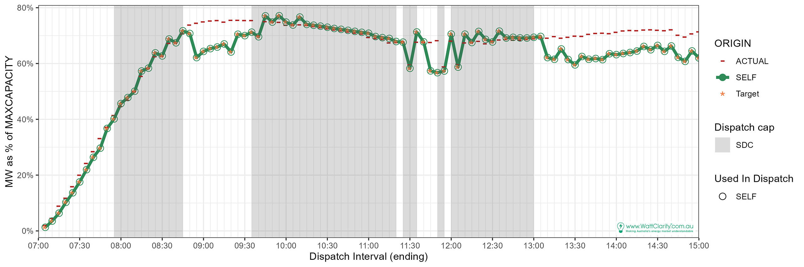
The notable biasing periods span the time ranges:

• Around 08:45 to 09:30,
• From 13:00 onwards,
• Some intervals around 11:45.

During those time ranges the self-forecast appears to be biased low, a fairly consistent 10% below the actual level of output. Actual output (actual) appears unmoved from what might be expected to be a more representative level of unconstrained output.

Let’s consider this self-forecasting behaviour according to the two legs of the game, noting that the biasing would be impacting on forecast performance:

Reducing regulation FCAS cost

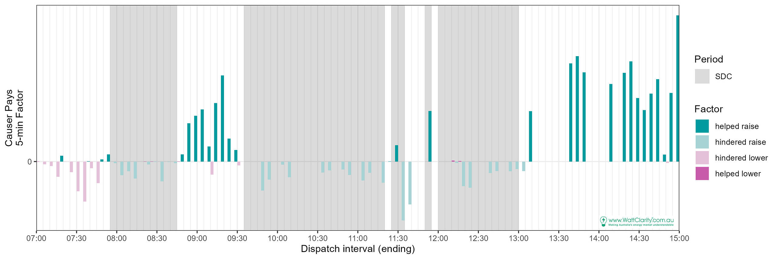
Below we present the factors. The 5-minute factors are eventually aggregated over a 4-week period allowing positive factors (helpful performance) to outweigh negative factors. Negative factors attract a share of the costs.

Predominately, the ‘biased’ intervals attracted positive raise factors, ‘helped raise’, and would therefore have helped to mitigate Regulation Raise costs. Particularly:

• Around 08:45 to 09:30,
• From 13:00 onwards.

Contribution to frequency is assessed via the FI

We know from past analysis that a unit’s MW performance (under the ‘Causer Pays’ method) is assessed against the Frequency Indicator (FI) for the unit’s impact on system frequency. And this drives the allocation of Regulation costs:

• In the article ‘Comparing Frequency Measures (Frequency, FI, FM)’ we explained the measures and their roles in some detail; and
• In the follow-on article ‘Three headline observations, about the use of proxies for System Frequency in Frequency Control mechanisms’ we explained the three key observations that readers should understand here.

The self-forecast biasing approach, in this case, appears to ‘work’ (if we define that as delivering a benefit to the DUID,  and ignore impacts to the system) because positive deviations align with positive FI periods.

‘Success’ depends on the FI being somewhat predictable for a full 5 minutes or longer, and the deviation having the same sign as the FI.

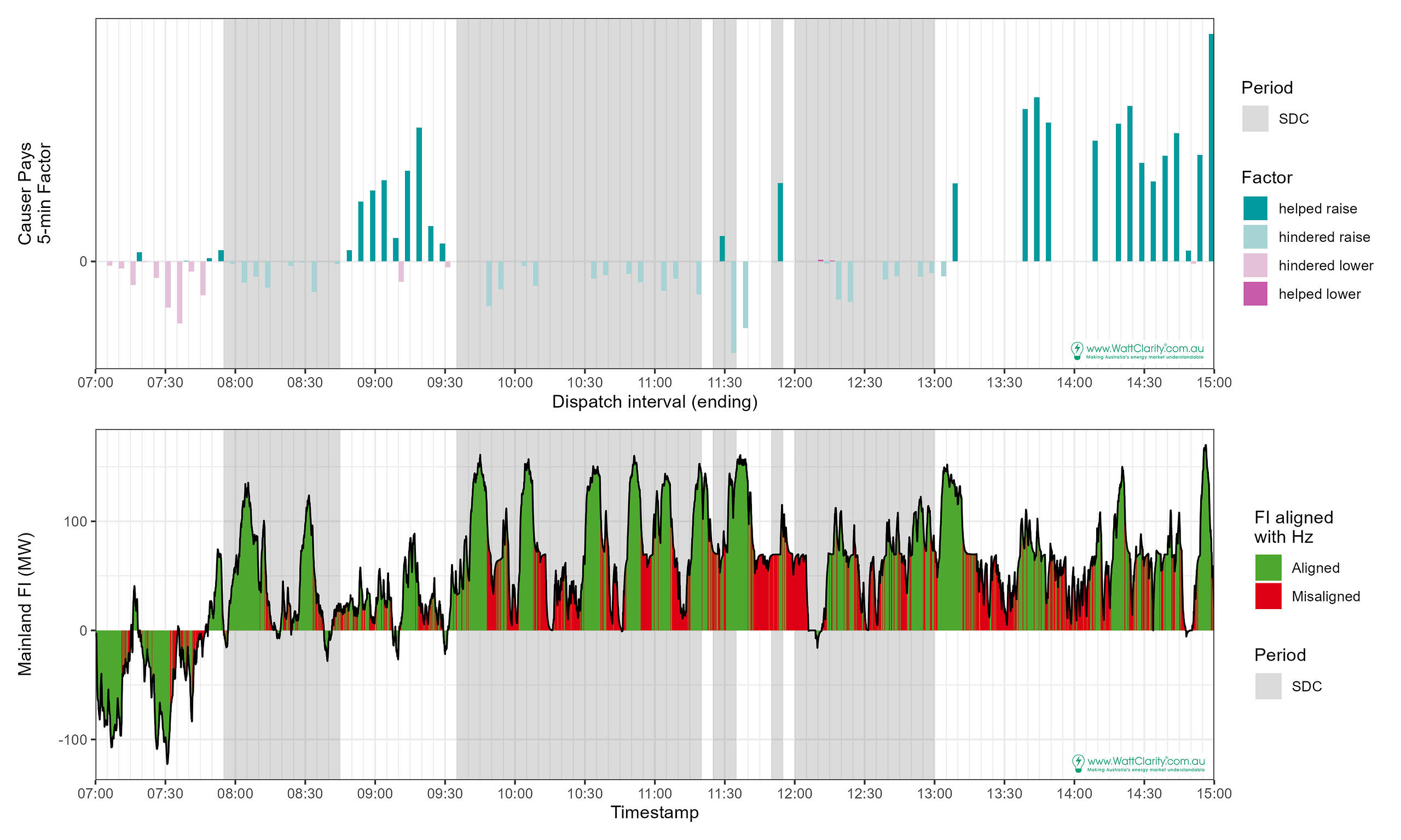
In our example, the FI (below, paired with the 5-minute factors chart from above) was almost always positive.  A positive factor may be earned when the FI and the unit-deviations have the same direction. Positive deviations help frequency raise.

Yet the FI needs also to be aligned with actual system frequency.

Positive factors not guaranteed

Positive factors (the approach ‘working’) aren’t guaranteed because:

Before the fact: A biasing direction (in this example, low) needs to be picked.

• • The resultant deviations might not be in the same direction as the FI.
    • Deviations could be evaluated as unhelpful.

After the fact:  A factor might not be able to be calculated, the effort could be of no value to the unit, and worse, negatively impact the system .

• • Frequency might be misaligned with the FI. The current ‘Causer Pays’ procedure tells us that the FI needs to be aligned with actual system frequency for the FI to be applicable.
    • We’ve noted before, and the chart shows, it can be misaligned often. FI was misaligned with frequency for almost 40% of 4-second periods through almost the whole of calendar 2024.
  • ‘Aligned’ periods are shown in green, in the chart above.
  • Where there aren’t enough green measurements, no factor is calculated. So that’s why some intervals didn’t earn a factor even when positive output deviations were occurring (e.g. 13:30).