Constraint Case Study Followup – Early outcomes of the new “X5 constraint”

Since the original Case Study on the newly-introduced N^^N_NIL_3 (or ‘X5’ ) constraint there have been several periods of this new constraint binding, directly affecting dispatch outcomes. This followup post examines its behaviour so far, and comments on other features of NEM constraints illustrated by this example that the first case study article didn’t have space for. Reading the original case study is strongly recommended before tackling this followup.

Binding behaviour

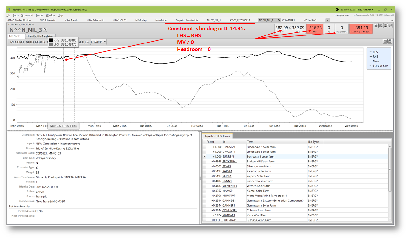
Here’s an ezview snapshot charting the N^^N_NIL_3 constraint’s behaviour – specifically its Left Hand Side (LHS) and Right Hand Side (RHS) values – on the day the first case study was published. As if to celebrate its newfound celebrity the constraint bound for quite a few Dispatch Intervals (Dis) from late morning through the afternoon of this day:

The next view – derived from AEMO’s underlying MMS data – shows a plot to the end of November of LHS and RHS values on the upper panel, along with the constraint’s Marginal Value (more on this below), while the lower panel shows contributions to the LHS from the various types of generation load and interconnectors involved in this particular constraint:

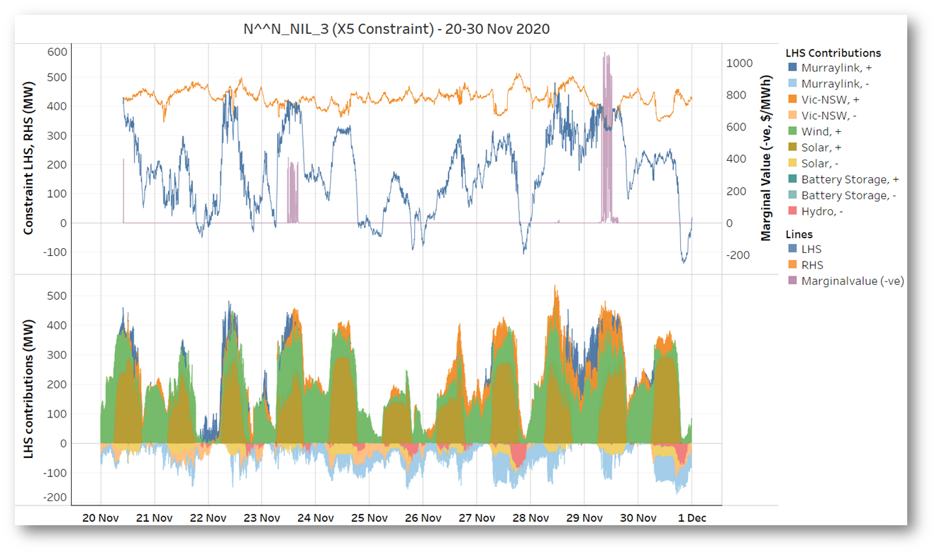
The constraint bound in 133 DIs, just over 4% of the period charted. Given the relatively large weighting of the constraint’s LHS towards wind and solar generators, it’s not surprising to see it only bind during daylight hours when wind generation was also significant, more or less as predicted in the original Case Study post.

This constraint has the form LHS <= RHS, and in DIs where it binds, AEMO’s dispatch algorithm NEMDE has had to make variations to one or more entities on the Left Hand Side (generator, load, or interconnector dispatch targets) to satisfy the constraint inequality. Indications that the constraint is binding are a headroom value of zero (headroom being just the difference between RHS and LHS), and a non-zero Marginal Value (MV). I’ll explain MV in more detail later, but it’s a measure of the constraint’s effect on increasing NEMDE’s least-cost dispatch objective.

Who’s affected?

Before grappling further with Marginal Value, let’s see if there are obvious impacts on the dispatch of entities on the Left Hand Side when this constraint binds. NEMDE’s optimization chooses the combination with least incremental cost to its overall dispatch solution. Here’s the full LHS again for reference:

 

As explained in the original case study, the incremental cost of LHS adjustments involves constraint coefficients, offer prices for generators and loads, and one or more regional spot prices. The overall size of the variation(s) NEMDE has to make clearly depends on how much the constraint would violate by if no changes were made, which is a function of the “unconstrained” LHS and any movements in the RHS (which comprises things that NEMDE can’t directly control).

I’m going to examine the 14:35 Dispatch Interval on 23^rd November which had a relatively large (negative) Marginal Value for N^^N_NIL_3. Here’s ez2view’s Unit Dashboard for Limondale 1 Solar Farm (“LIMOSF11”), which appears on the constraint LHS with a coefficient of +1.000:

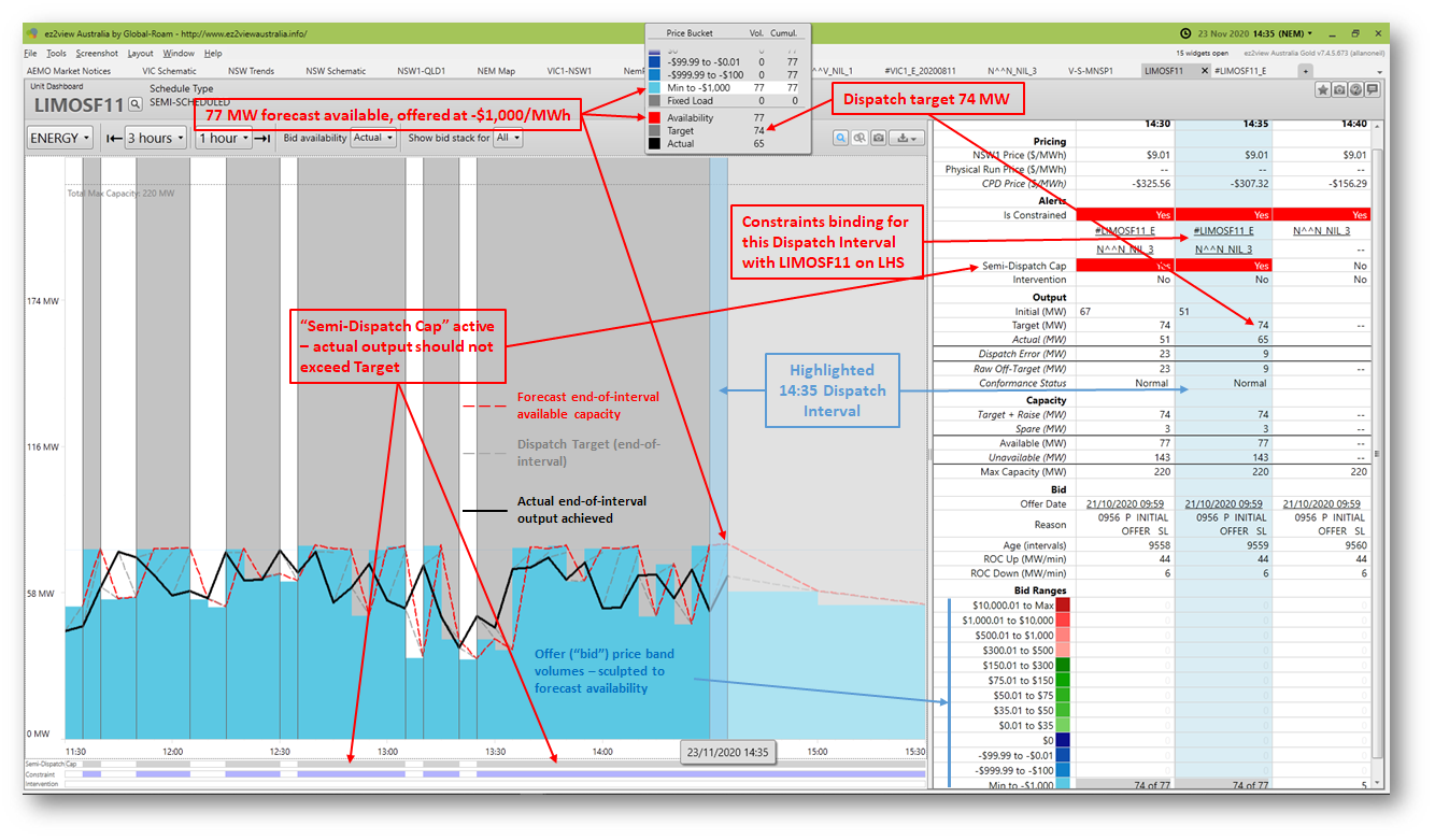
There’s a LOT of information on this ez2view widget. Key features relevant to possible constraint impact are highlighted. The following comments may aid interpretation:

• Because this is a semi-scheduled solar generator, available output varies minute by minute with sunlight conditions, so forecast availability and achieved actual outputs
  • jump around between dispatch intervals (this was probably an intermittently cloudy day);
  • don’t coincide particularly closely – even over five minutes, forecasting sunlight levels is difficult!
• All available output – as limited by this varying sunlight – was being offered at negative $1,000/MWh. The original case study explained that within NEMDE’s optimization the lower a generator’s offer price, the higher the “cost” to optimal dispatch of reducing its output, all other things being equal, so the lower the chance of its output being restricted. Limondale appears to be offering its energy with this issue in mind.
• NEMDE’s dispatch targets for a generator offering like this will – unless reduced to satisfy a constraint – almost always follow availability, as shown by the dashed grey line (end-of-interval targets) rising or falling to the dashed red line (forecast end-of-interval availability).
• In DIs where a semi-scheduled generator is part of a binding constraint, its dispatch targets should be treated as caps on actual output, indicated by the Semi-Dispatch Cap flag, active even if NEMDE has not adjusted target output to below forecast availability. This is intended to ensure that the constraint is not breached by a semi-scheduled generator able to produce more energy than forecast for the DI (hawk-eyed observers might note several earlier DIs in the chart where Limondale has apparently failed to follow this obligation).
• In the highlighted 14:35 interval – and others where the same highest availability of 77 MW is forecast – the NEMDE dispatch target is just lower at 74 MW. Is this the impact of the N^^N_NIL_3 constraint?

No. There are actually two binding constraints indicated for this interval, and it’s not N^^N_NIL_3 but the #LIMOSF11_E constraint which lowers the dispatch target in the 14:35 DI (and others where the same 77MW availability is forecast):

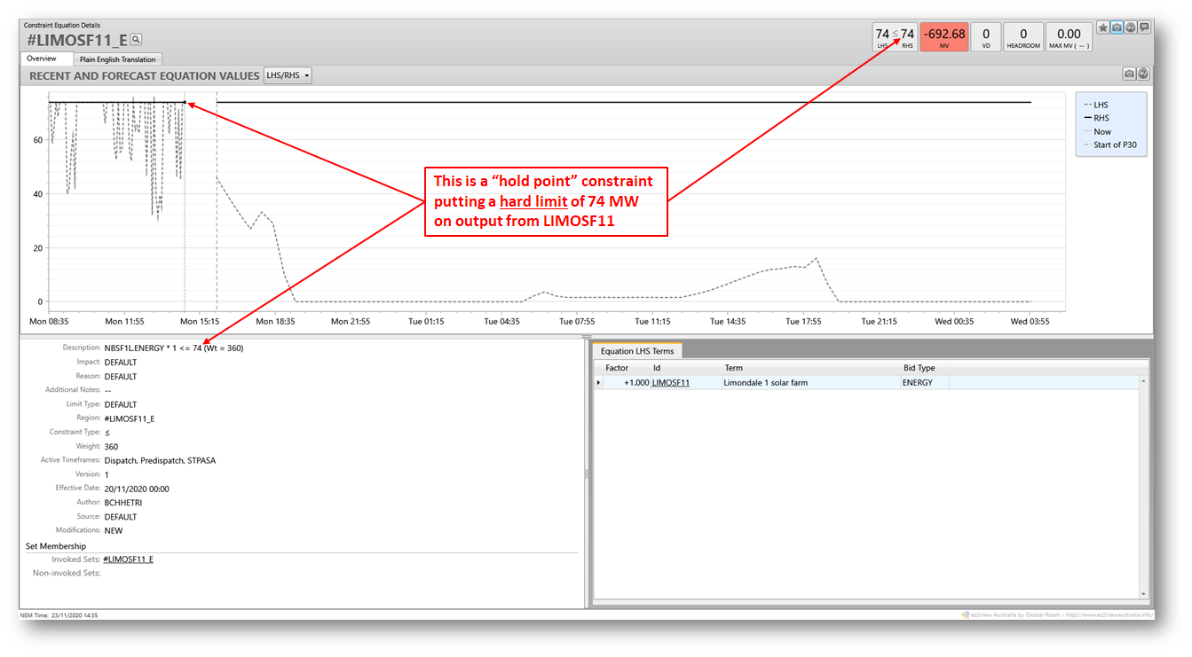
Limondale 1 is a solar farm still in its commissioning phase, with about one third of its full capacity in service, and it’s relatively common for generators in this phase to be subject to hold point constraints on maximum output while various commissioning and testing activities proceed.

So a bit of a digression onto a different constraint, but another illustration of how constraints are used in NEM dispatch – in this case simply to put a ceiling on an individual generator’s output.

Getting back to N^^N_NIL_3, similar examination of other generators and loads on its LHS confirms that their dispatch targets were not adjusted to satisfy this constraint, on this particular day at least.

A look at interconnectors

That leaves the two interconnectors on the LHS of the constraint. Here it’s worth stepping back for a look at the overall dispatch picture in DI 14:35

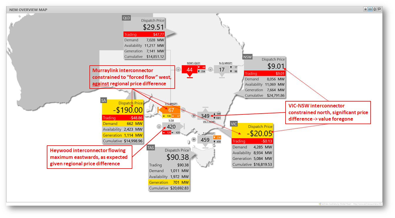
This highlights immediately the impact that something – perhaps N^^N_NIL_3 – seems to be having on flows across these two interconnectors: the VIC-NSW AC interconnection, and the Murraylink DC cable (“V-S-MNSP1”) linking the Riverland regions of Victoria and South Australia. We see immediately that:

• Murraylink is being forced to flow from (relatively) higher priced Victoria (spot price -$20.05/MWh) to lower priced South Australia (-$190/MWh). The 67 MW shown flowing westwards is the dispatch target for this DI, on which the economic loss would be roughly $11,000 per hour (ignoring any energy loss impacts).
• Flows from Victoria to NSW are being limited to a 349 MW target, despite a price difference of nearly $30/MWh. An additional 100 MW of northerly flow would reduce NEMDE’s dispatch costs by about $3,000 per hour.

These are both significant impacts on dispatch. Interconnections usually transfer energy from lower priced to higher priced regions, up to a level where the cost of energy losses on higher transfers would exceed the regional price difference, or a physical or security limitation prevents higher flows. The counter-price flow on Murraylink is prima facie uneconomic, and there is also economic value being foregone on Victoria to NSW flows.

So how do we confirm that this is all the work of N^^N_NIL_3 and not some other constraint?

First of all ez2view tells us, using information published in the market dispatch data:

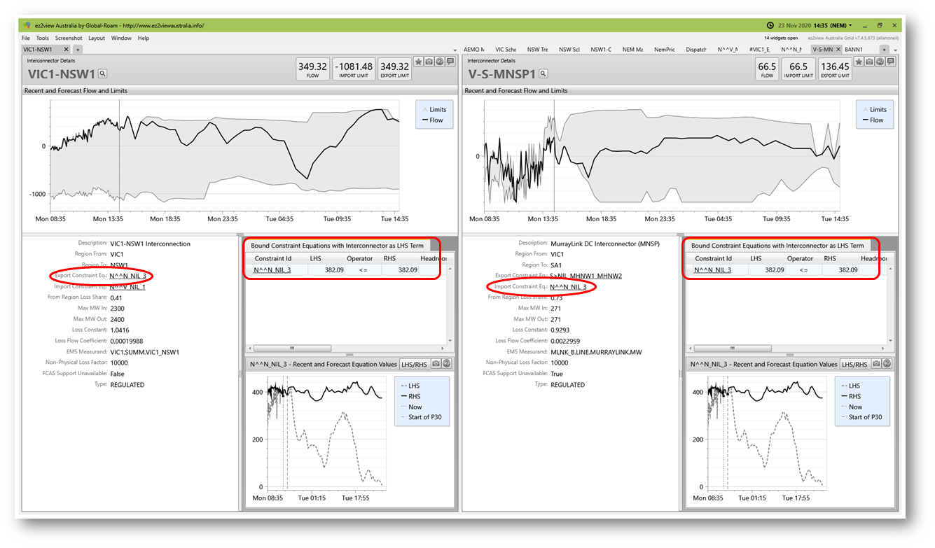
The summary for each interconnector lists N^^N_NIL_3 as the only binding constraint in this DI with that interconnector on its LHS. Had there been additional binding constraints, one or more of these might affect dispatch targets before N^^N_NIL_3 (analogously to Limondale 1 solar farm’s hold point constraint).

The original case study also explained why generators which might be constrained down by a binding constraint have incentives to offer output at very low prices – such as the negative $1,000/MWh offered by Limondale. Interconnectors appearing in the same constraint may then become “first cab off the rank” for adjustments to target dispatch levels. That seems very likely to be what’s happening here.

We can dive a little deeper into the principles used by NEMDE to solve the problem of satisfying the constraint, and demonstrate that the cost to dispatch in constraining each interconnector is very precisely balanced between the cost of counter-price flows on Murraylink and the restriction on profitable flows from Victoria to NSW. The exercise also reveals exactly what the constraint Marginal Value number means. But this gets very detailed, so by all means jump on to the following section if you prefer.

A detailed look at interconnectors – and Marginal Value (* maths alert *)

Let’s examine what it “costs” NEMDE to achieve a 1 MW reduction on the LHS expression of N^^N_NIL_3 in the 14:35 DI. To satisfy the constraint inequality, NEMDE must reduce the LHS when it would otherwise be too high.

First take the VIC1-NSW1 interconnector which has a LHS coefficient of +0.09287. Flows from Victoria to NSW count as positive, so to reduce the LHS by 1 MW by varying the flow target for this interconnector requires a target variation of -1 MW / 0.09287 = -10.77 MW. This flow reduction is consistent with the constraint “holding back” profitable transfers from Victoria (-$20.05/MWh) to NSW ($9.01/MWh).

In the original case study the cost (per hour) for varying this interconnector target was shown as

[change in target MW (-ve for reduction)] * ([Vic spot price $/MWh] – [NSW spot price $/MWh])

(Ignoring any changes in inter-regional losses for simplicity)

It’s fairly easy to see that this is the “opportunity cost” of Vic -> NSW exports foregone in order to reduce the constraint LHS by 1 MW. The calculation yields:

[-10.77 MW] * (-$20.05 – $9.01)/MWh = +$313.0 per hour

But it’s possible to be more precise and include the impact of changing losses. Without going into its derivation, the extra term relating to changes in interconnector losses is

[change in target MW (-ve for reduction)] * [interconnector marginal loss factor – 1]
* WtdAvg([Vic spot price $/MWh], [NSW spot price $/MWh])

The “WtdAvg( )” expression is the average of Victorian and NSW spot prices, weighted by AEMO’s inter-regional loss proportions for the interconnector. This proportioning is fixed annually for each interconnection path and for the Vic-NSW interconnector it’s currently Vic 41.45%  / NSW 58.55%. The “interconnector marginal loss factor” is a dynamic parameter varying between Dispatch Intervals – depending principally on the flow level across the interconnection – but fortunately its value is published every DI for each interconnector. For the 14:35 DI its value for VIC1-NSW1 was 1.11819. With these data in hand the contribution of changed losses to the hourly cost of NEMDE’s flow adjustment is calculated as

-10.77 MW * (1.11819 – 1) * (0.4145*(-$20.05) + 0.5855*$9.01)/MWh

= -10.77 MW * 0.11819 * (-$3.0354/MWh) = +$3.863 per hour

For anyone following closely: reducing the northerly flow on this interconnector also reduces physical energy losses, but this increases the cost NEMDE sees for the flow adjustment because the negative spot price in Victoria means smaller losses in that region are a net cost to dispatch!

Adding together the two values just calculated yields the net hourly cost to dispatch of achieving a 1 MW reduction of the constraint LHS by reducing flows on VIC1-NSW1:

+$313.0 + $3.9 = $316.9

On Murraylink, with a coefficient of -0.5197, a reduction of 1 MW to the constraint LHS requires a change in flows of -1 MW / -0.5197 = +1.924 MW. For this interconnector, this means an increase in westerly flows which are counted as positive. The cost to dispatch ignoring losses is

+1.924 MW * (-$20.05 – (-$190))/MWh = +$327.0 per hour

The loss expression, using the appropriate values for Murraylink and SA in this DI, is

1.924 MW * (1.08624 – 1) * (0.7296 * (-$20.05) + 0.2704 * (-$190))/MWh

= 1.924 MW * 0.08624 * (-$66.00/MWh) = -$10.95 per hour

Here there are higher physical energy losses with increased westerly flow but this reduces the net dispatch cost because of the negative prices in both Vic and SA. Bizarre.

So the overall hourly cost to dispatch of this change in Murraylink flow is

$327.0 – $10.95 = $316.1

In summary, we’ve calculated that in this DI, achieving a 1 MW reduction on the constraint LHS:

• by reducing Vic-NSW flows (by over 10 MW) would cost $316.9 per hour, or
• by increasing Murraylink Vic-SA flows (by just under 2 MW): $316.1 per hour.

So in satisfying the constraint NEMDE has found a neat balancing point for flow adjustments across the two interconnectors which equalizes their marginal impact on dispatch costs; this is actually a necessary condition of finding the optimum dispatch solution.

Finally, it’s no coincidence that the marginal value (MV) of the N^^N_NIL_3 constraint in this DI is reported by NEMDE as -316.33 – because the marginal value of any constraint is defined as the change in hourly dispatch cost if the constraint RHS (and hence the LHS if the constraint is binding) were increased by 1 MW. This negative value is just the opposite of the marginal cost increases found above for reducing the LHS by 1 MW.

(And while Marginal Value may still seem esoteric, NEM spot prices themselves are simply the marginal values found by NEMDE for internal constraint equations which specify that Supply = Demand.)

This may all be very satisfying mathematically, but it’s worth stepping back now and reflecting on the physical and economic implications of the constraint’s behaviour.

What’s the overall impact and cost of the constraint?

There’s no simple way to work out a binding constraint’s total impact on dispatch, unlike its marginal impact. NEMDE would have to be re-run with the constraint removed and differences in dispatch quantities and prices then analysed. For our purposes we can get a rough idea by looking at the dispatch outcome twenty minutes later in DI 14:55 when the constraint was no longer binding. Other things have changed in the meantime, but changes in flows on the two affected interconnectors and (with somewhat less certainty) changes in SA and Vic spot prices give a sense of the overall impact the N^^N_NIL_3 constraint may have been having in the earlier DI:

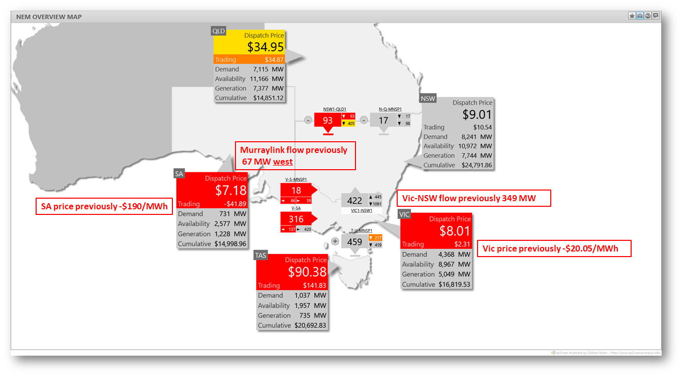
The summary shows

• increased flows on the Vic-NSW interconnector – previously “held back” to satisfy N^^N_NIL_3
• flows on Murraylink are now from lower to higher price – previously being forced westwards against a large price difference
• spot prices in SA, Vic and NSW are closely linked, with differences reflecting only interconnector marginal losses, not constraint impacts

When binding, the N^^N_NIL_3 constraint was affecting both interregional flows and almost certainly prices in both Victoria and South Australia. This might not seem too peculiar, but as outlined in the original case study the purpose of the constraint is to limit flows on a single specific transmission line in NSW, the X5 line from Balranald to Darlington Point. So it is perhaps surprising that satisfying the constraint has caused fairly wide-ranging impacts across multiple regions.

Here’s a highly schematic view of the NSW system, reproduced from the original case study, showing location of the X5 line and in addition zones in NSW and Victoria containing generators that tighten the constraint (positive LHS coefficients) and ease it (negative coefficients):

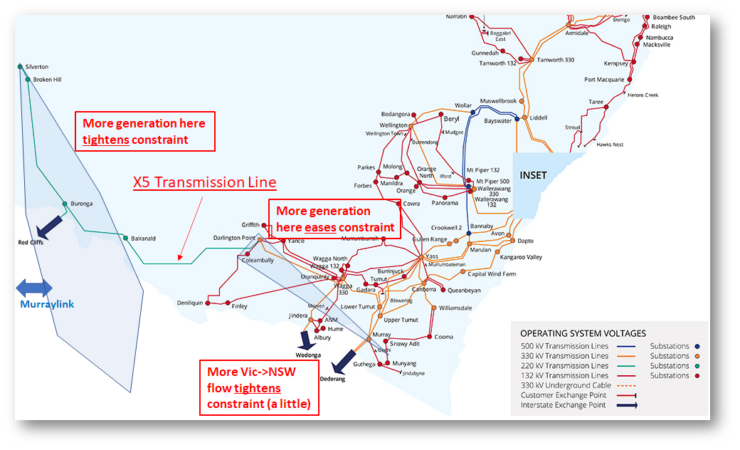
Generators in the extended “rhombus of regret” to the west of the X5 line have positive constraint coefficients. A few generators to the east of the X5 line have negative coefficients and ease the constraint if running. Because Murraylink connects into the “rhombus”, its negative coefficient on westward flows is equivalent to a positive coefficient when flowing east and adding to generation in the rhombus.

Intuitively, this all makes sense, but why do overall Vic to NSW transfers enter the constraint equation with a small positive coefficient? Because Victoria and NSW connect through the “rhombus” zone as well as much more directly through Snowy & Wagga, and a small proportion of any overall Vic – NSW transfer effectively takes the long route through Red Cliffs & Buronga, contributing to additional flow on the X5 line.

The constraint coefficients mean that to satisfy the X5 constraint when it’s binding, NEMDE’s dispatch algorithm has four basic choices:

1. constrain downwards one or more generators in the “rhombus”
2. constrain upwards one or more generators immediately east of the X5 line
3. reduce easterly / increase westerly flows on Murraylink
4. reduce northerly / increase southerly flows between Vic and NSW

Considering only physical impacts on dispatch – the MW amounts by which generation or interconnector targets would need to be altered – then the first option of winding back generators with the largest positive coefficients has the smallest impact. A 1 MW reduction at Limondale yields a 1 MW change in constraint LHS. Adjusting Victoria to NSW interconnector flows requires a 10.77 MW reduction to achieve the same LHS reduction. But NEMDE follows an economic optimization: when Limondale (and other generators) offer their energy at -$1,000/MWh, NEMDE will almost certainly find a “cheaper” solution involving significant changes to flows on two interconnectors, with consequent impacts on regional spot prices.

Does this really make economic sense?

It does within the optimisation framework given to NEMDE, but the example highlights a side-effect of the NEM’s region-wide spot pricing model. Whether affected by the constraint or not, generators in a given NEM region all receive the same spot price (adjusted by their Marginal Loss Factors). By offering at -$1,000/MWh, generators that would potentially lose volume under a constraint may avoid being wound back, and perhaps insulate themselves from the constraint’s effects. This behaviour – quaintly known as “disorderly bidding” – can, depending on the specifics of the relevant constraint, force the market dispatch algorithm to choose a much more “physically disruptive” dispatch solution with possibly wider financial flow-on effects.

Under a nodal spot pricing model, constraint marginal costs would be directly reflected in location-specific spot prices paid to generators at affected nodes. The higher the marginal cost of a constraint and the larger a generator’s constraint coefficient, the greater the impact on the nodal spot price. This model would result in quite different bidding and dispatch outcomes. In the case of the physical limitation underlying N^^N_NIL_3, nodal pricing would almost certainly concentrate the changes in dispatch targets amongst the high-coefficient generators.

Whether a regional or nodal pricing approach is preferable for the NEM raises many wider issues than their relative effects on constraint impacts and dispatch patterns. There may also be pragmatic ways to adjust constraint formulation that could partially address some side effects of “disorderly bidding” (eg removal of interconnectors with small LHS coefficients) without any wider changes to NEM dispatch and pricing arrangements.

The point of this case study was certainly not to make an argument one way or the other for what would be a very substantial change to NEM architecture, but it’s interesting to see how examining the micro-detail of a single constraint’s operation and outcomes can lead to much wider questions about the structure within which that constraint operates.

 

---

About our Guest Author