
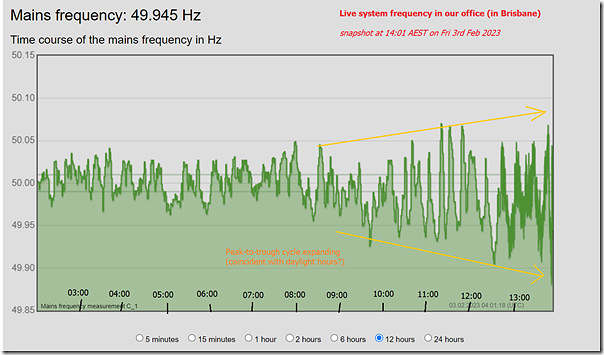
There were many posts here on WattClarity last Friday – almost a live blog – as Queensland demand appeared headed for record territory. A cool(er) change put paid to that, much to the relief of many Queenslanders and probably power system operators as well. But amidst the focus on peak demand and supply reliability, Paul noticed some wobbles in the system frequency – a real-time indicator of instantaneous supply-demand balance – and put up a short post which also prompted some discussion on LinkedIn. I’ve reposted his central chart below:
With key outcomes for the day already well documented and discussed, I thought it would be interesting to dive a little deeper into the frequency movements noticed by Paul, to look for any clues on their origin. While there were no large excursions of the kind seen when there is a major system contingency, there were enough fairly rapid shifts, with some occasional five-minute periodicity in the movements, to make me wonder if it was related to the dispatch performance of market generators – in other words an artefact of the NEM’s five minute market dispatch process.
Quick refresher – how are supply and demand balanced in the NEM?
For readers unfamiliar with some of the detail and terminology I’m going to use, this is a short summary of how supply and demand stay in balanced in the NEM – not at all comprehensive.
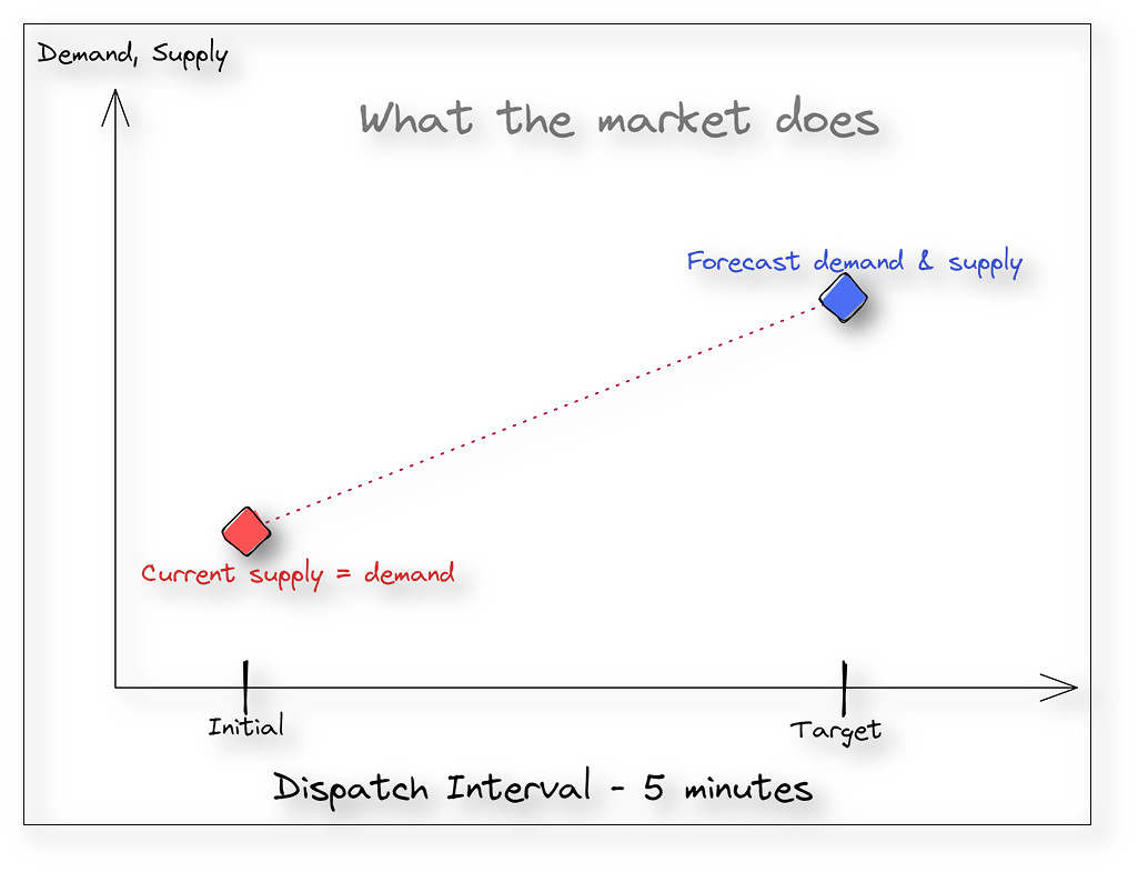
Market processes in the NEM target supply-demand balance solely at 5-minute dispatch interval (DI) boundaries, and only as a forecast outcome. The market dispatch process “knows” where supply and demand sit at the beginning of each DI thanks to real time SCADA metering feeds from all large-scale generation and scheduled load units across the grid. The process then allocates new dispatch targets across this fleet that would balance wholesale supply with forecast demand in five minutes’ time, at the end of each interval. Units whose outputs would change are expected to ramp to their new target following a linear path – but this does not mean that the dispatch process explicitly forecasts a smooth linear trajectory for demand.
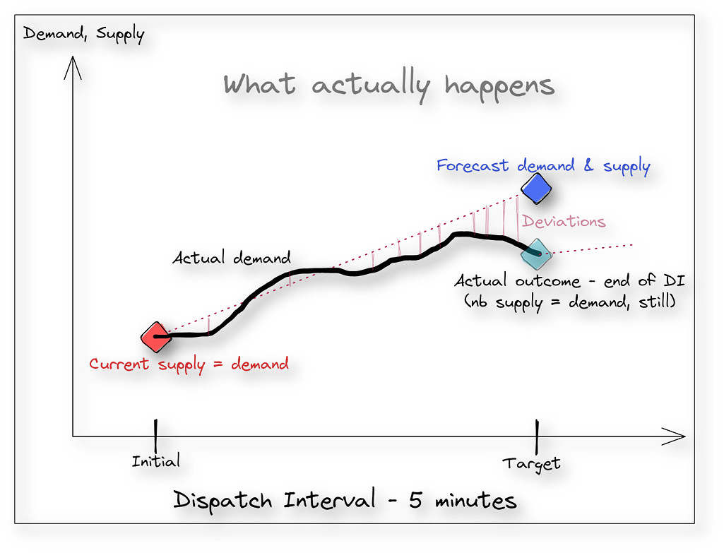
The reality of any power system is that demand can move much more erratically at second-to-second granularity than a linear ramp – or any forecast trajectory – implies. The market operator’s end-of-DI demand forecasts are rarely spot-on. Nor do dispatchable generators and loads always follow linear output trajectories, or even achieve their allocated market dispatch targets at the end of each interval. So on both the demand and supply sides there are inevitable deviations – sometimes large ones – away from the simple market view summarised above.
The job of maintaining real-time supply-demand balance therefore falls not to the market, but to much faster acting frequency control mechanisms. Why frequency? – because movements in system frequency away from the nominal 50 hertz level reflect real-time imbalances between aggregate supply and demand. The mechanisms most relevant to this article are Primary Frequency Response (PFR) and Regulation FCAS. These both involve processes – controlled changes in unit output or scheduled demand levels in response to frequency movements – which aim to steer system frequency back towards 50 hertz after deviations on the demand or supply side nudge it away.
Frequency Last Friday
To recap the frequency movements we’ll be looking at from February 3rd, here’s another chart of mainland NEM frequency, drawn from AEMO’s 4-second granularity causer pays dataset.
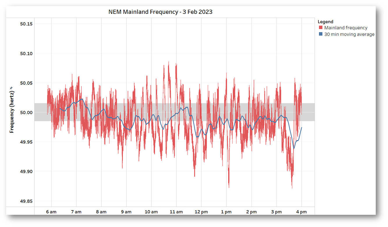
The shaded grey region between 49.985 Hz and 50.015 Hz (+/- 0.03% from 50 Hz nominal) is the Primary Frequency Response ‘deadband’ – outside this narrow range most NEM generators are expected to respond so as to resist frequency deviations (if technically able to do so). While the frequency last Friday was wandering within and around this deadband, it was clearly contained well within the Normal Operating Frequency Band of 49.85 to 50.15 Hz. However as Paul noticed, from around 9am we can see larger amplitude variations in frequency starting to appear, some with a more cyclical character.
The 30 minute moving average also shows that through much of this daytime period, average frequency tended to the low side of 50 Hz and was less contained within or near the PFR deadband.
Solar Focussing
One of Paul’s suggestions about these larger daytime variations was that they might reflect some characteristic of solar generation. As we know the NEM has two different forms of solar generation, both very significant:
- Distributed (rooftop) PV systems which in aggregate comprise something approaching 17 GW of capacity in the NEM, installed across millions of homes and businesses. Real-time total output from these systems is not visible to the market – although both AEMO and the Australian Photovoltaic Institute (APVI) maintain fairly sophisticated systems, based on sampling and/or solar irradiance measurements, for estimating their aggregate actual output at granularities of ~5 to 30 minutes. This output effectively subtracts from the total grid demand to be supplied from the wholesale market.
- Grid-scale (utility) solar farms with aggregate capacity of about 6.5 GW. Unlike rooftop systems, most of these farms are dispatched through the wholesale market and real-time SCADA output data is available down to individual farm level at 4 second granularity.
Without accurate high-resolution data on aggregate rooftop PV output it’s hard to analyse whether short-term variability in this source (playing out as NEM demand variability) might be a factor in driving frequency deviations. In looking for any trends I’ve therefore confined my analysis to the second category of grid-scale solar generation.
One hypothesis about how solar output variations might impact system frequency is that relatively sudden drops or jumps in output (passing cloud cover etc) could lead to short term supply-demand imbalances and cause system frequency to deviate until frequency control mechanisms like PFR and Regulation FCAS act to correct it. A variation on this hypothesis is that these output changes are unexpected and therefore not forecast within the dispatch process – changes in output that are forecast within the market dispatch timeframe should be accommodated through appropriate setting of other units’ dispatch targets.
We’ll also look at output profiles from other forms of generation for any clues about or responses to frequency movements. But first it might help some readers to have a few more details about how “intermittent” energy generators like solar and wind farms are dispatched in the market.
How are intermittent solar and wind generators dispatched in the NEM?
Forecasting the 5 minute ahead availability (maximum output) of large scale solar and wind generators is an important part of the dispatch process. AEMO forecasts dispatch availability for all “semi-scheduled” solar and wind generators in the NEM every five minutes. Participants can also submit their own self-forecasts. Dispatch targets for these generators can be set below forecast availability:
-
-
- Where they have offered some or all available capacity at prices equal to or above the spot price – “economic offloading”
- If lower levels of output are required because of transmission or other system security constraints – “curtailment”
-
In intervals where a semi-scheduled generator is not offloaded or curtailed, its dispatch target is not a binding limit on output – if more power is available within the dispatch interval it is not prevented from increasing output above the target. However in intervals where it is offloaded or curtailed (or even when not curtailed, if the generator ccontributes to a constraint which is binding) a semi-scheduled generator is subject to a semi-dispatch cap (SDC) which means it should not generate at higher levels than its dispatch target.
Whether or not a SDC applies, a semi-scheduled generator should not cut output below its dispatch target where it has sufficient wind or solar resource available to meet that target. As with other generators, wind and solar generators are also generally expected to follow linear ramps between dispatch targets, to the extent that available wind or solar resources allow them to do this. These obligations were introduced partly in response to events where some semi-scheduled generators were immediately switching off in response to large negative spot prices: even if it receives a dispatch target of zero in response to such a price, a semi-scheduled generator is expected to ramp down linearly to that target, not immediately cut its output to zero.
Dispatch Performance
Here’s the central chart in this investigation – showing the 4-second aggregate output profile of the NEM’s grid-solar farms across the main daytime period, plotted against their aggregate 5-minute dispatch targets and availability levels. Underneath is the corresponding mainland frequency trace. I’ve highlighted most of the periods where frequency took a dive towards lower territory within the NOFB. In a separate colour I’ve highlighted a period of frequency swings between about 10:15 and 11:05 which we’ll look at in a little more detail later.
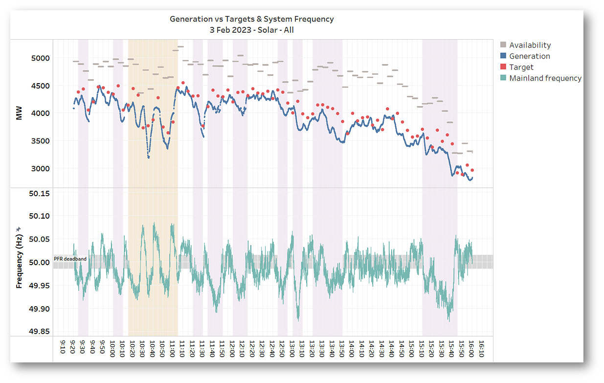
Humans are prone to seeing patterns in randomness, but I’d still venture the following observations based on this chart:
- There’s a surprising amount of output variability – this reflects both forecast changes in resource availability from DI to DI (the grey line segments), but also varying amounts of curtailment and offloading (represented by the gap between availability and the dispatch targets shown as red points at the end of each DI).
- Additional variability arose from aggregate solar output often missing its end of interval dispatch targets – typically on the low side, with a maximum difference of nearly 600 MW.
- Periods of lower system frequency do appear correlated with relatively large deviations between dispatch targets and actual output, and also with periods where solar output was declining rapidly.
- Conversely, in the 10:15-11:05 am period we also see some higher frequency events coinciding with periods where solar output was rising rapidly, and in a few intervals exceeding its end of interval dispatch target.
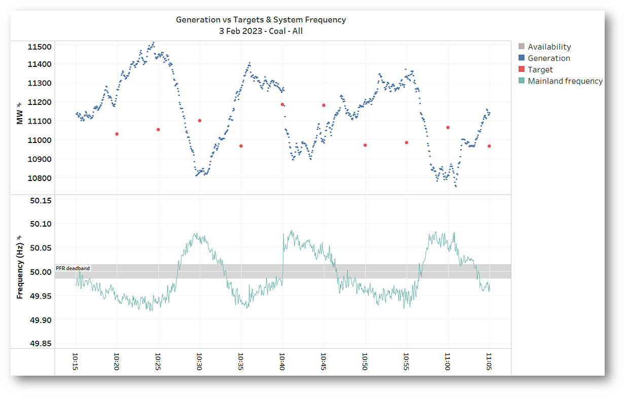
What about other generation types? Here’s a similar picture for the NEM’s operating coal units – I’ve suppressed the availability lines here which are up around the 17 – 18 GW level
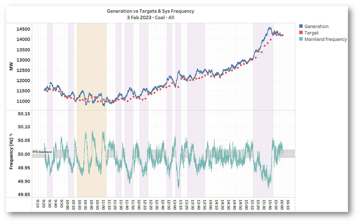
Here we can very clearly see a pattern of output deviations from target which correlate inversely with frequency levels: output above targets when frequency is low, and below targets when frequency is high. I’d suggest that a lot of this reflects Primary Frequency Response in action, since these deviations are directionally what generators delivering PFR are expected to do. In effect, coal generation output is moving away from its targets in a controlled fashion to counteract the opposite “unexpected” deviations in large solar output (and possibly other factors), with system frequency being the co-ordinating signal.
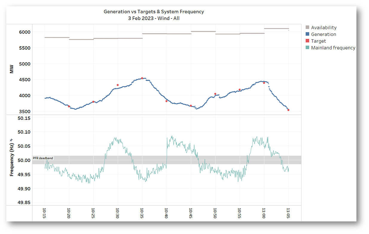
What about wind generation?
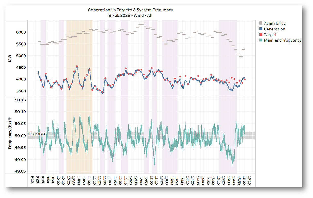
Quite an interesting picture, with the following observations:
- There’s a significant amount of offloading and curtailment reflected in the gap between windfarm availability and dispatch targets. Without doing a detailed analysis I’d suggest a lot of this is price-based offloading rather than forced curtailment – spot prices were low through much of the day, especially in the southern regions which host the majority of the NEM’s wind capacity.
- Variability in dispatch targets and output was at times – particularly early in the day – much larger than changes in availability: indicating changing amounts of offloading and curtailment, again most likely to reflect price-based offloading.
- Wind in aggregate did a much better job than large solar in following its dispatch targets, and except in one isolated set of intervals (around 3:20 – 3:40 pm) rarely fell far below targeted output.
- There’s little sign of windfarms materially responding to frequency excursions – I haven’t checked, but it looks like windfarms are not (yet) enabled to deliver PFR
Summing Up
This has been only a high level scan of events contributing to frequency deviations on the day analysed (and for all I know similar deviations could be happening most days), but the evidence does suggest challenges in accurately forecasting grid-scale solar output even at the relatively short timescale of the NEM’s five minute dispatch process. A deviation of 600 MW over a single dispatch interval is equivalent to loss of a large traditional generating unit. While the NEM’s frequency control mechanisms are well set up to manage this level of variability, continued growth in large scale solar capacity will only increase the challenge.
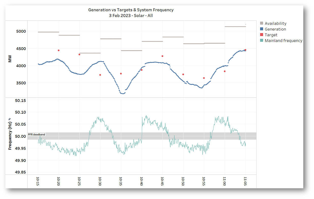
Postscript – Diving Slightly Deeper
To finish, a few more charts taking a closer look at the period of frequency swings between 10:15 am and 11:00 am that I think first prompted Paul’s original post. Aggregate solar dispatch in this period, where it’s easier to pick out the deviations above and below dispatch targets:
Coal – showing its countercyclical PFR response:
Wind – following its varying dispatch targets nicely:
In looking deeper into solar farm behaviour in this period a few interesting artefacts popped out. While not comprehensive and certainly not intended to “name and shame”, the following couple of examples illustrate some broader issues touched on above.
One of Queensland’s largest new solar farms, Western Downs, appears to have been doing some testing, rapidly ramping down and then back up by 75 MW, 185 MW and 330 MW over five dispatch intervals:
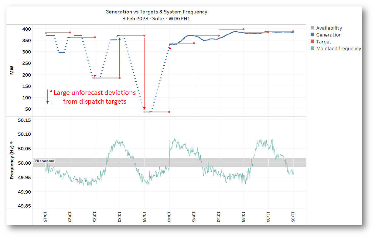
The only issue with this is that AEMO’s dispatch process – in particular its availability forecasts across the period – appeared to know nothing in advance about these movements, resulting in the highlighted large gaps both ways between dispatch targets based on those forecasts and actual output from the solar farm. With deviations of over 300 MW this doesn’t seem ideal, and would certainly have been a factor contributing to the frequency swings Paul commented on.
In a few other cases, we can see solar farms that didn’t always follow linear ramps between dispatch targets. One of them was Bluegrass solar farm, also in Queensland:
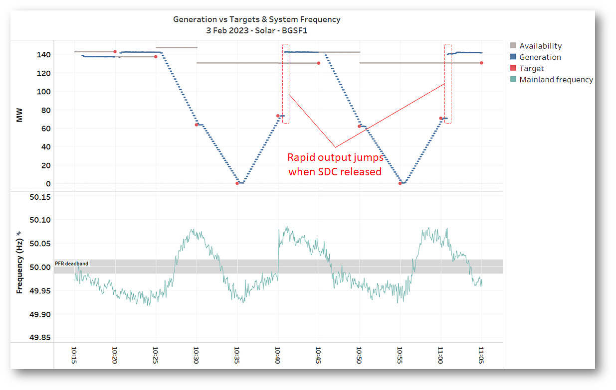
When subject to a semi-dispatch cap (where its output target was below availability – almost certainly based on its offer pricing), the farm’s output profile follows nicely controlled linear ramps between targets. But in the DIs starting at 10:40am and 11:00 am we can see that its end-of-interval dispatch target goes back to maximum availability – meaning no semi-dispatch capping – and the farm’s output immediately jumps to an uncapped level, with no ramping at all. While these 80 MW jumps by themselves are not a huge problem, they might become one if dozens of farms behaved similarly all at the same time!
=================================================================================================
About our Guest Author
 |
Allan O’Neil has worked in Australia’s wholesale energy markets since their creation in the mid-1990’s, in trading, risk management, forecasting and analytical roles with major NEM electricity and gas retail and generation companies.
He is now an independent energy markets consultant, working with clients on projects across a spectrum of wholesale, retail, electricity and gas issues. You can view Allan’s LinkedIn profile here. Allan will be ocassionally reviewing market events here on WattClarity Allan has also begun providing an on-site educational service covering how spot prices are set in the NEM, and other important aspects of the physical electricity market – further details here. |
Leave a comment