Examples of self-forecasting behaviours – under the hood of part 1

In Part 1 we shared an example of self-forecast biasing that underpinned positive unit MW deviations relative to target.

Those positive deviations led, sometimes, to helpful Causer Pays factors at the 5-minute level. These helpful factors (until June 8 2025) go towards reducing regulation FCAS costs, this being the assumed motive behind the biasing.

From June 8 2025 the approach to Regulation FCAS cost recovery is different with the introduction of Frequency Performance Payments.

Why the 5-minute factors don’t always reflect the deviations

In Part 1 we looked at an anonymised unit’s sequence of daytime intervals (7am to 3pm).

We found helpful factors (the approach ‘working’) aren’t guaranteed through self-forecast biasing.

Some reasons were given for why in the Part 1 article. In this digression we unpack reasons for the mixed results using 7 dispatch intervals from that afternoon.

Our example zooms in on seven intervals

Those 7 intervals are highlighted in the red box:

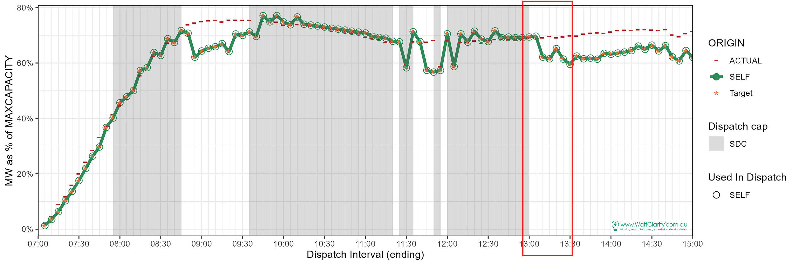
Zooming in, we verify that targets match the self-forecast. Biasing-low is visible from the 13:10 interval onwards.

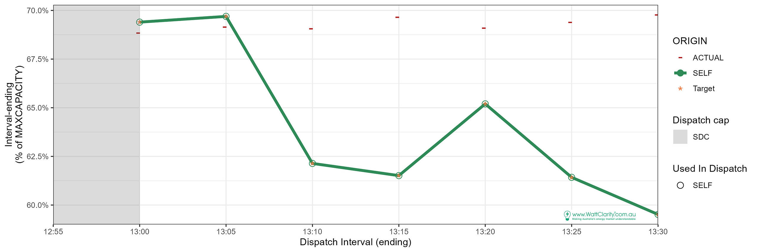
Yet dispatch interval-ending performance isn’t enough to assess frequency impact.

For evaluation against frequency, unit MW measurements every 4 seconds are used.

Unit output deviations at 4-second cadence

The difference between target MW and output MW forms the basis for a unit’s contribution to frequency performance.  We see positive deviations in the green-shaded range which contribute a frequency-raising effect.

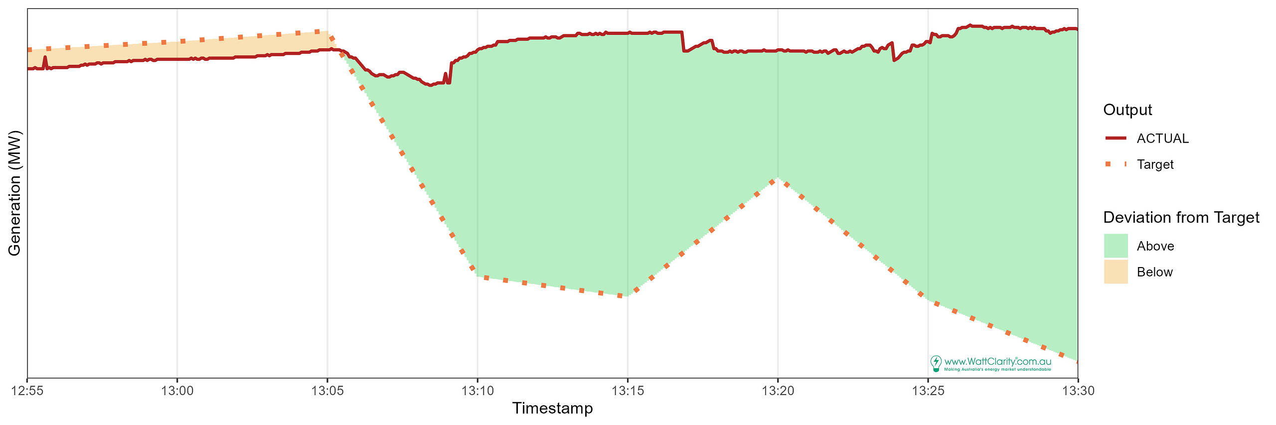
From Part 1’s discussion we recall that deviations primarily need to be in the same direction as the Frequency Indicator (FI).

Frequency indicator alignment is necessary

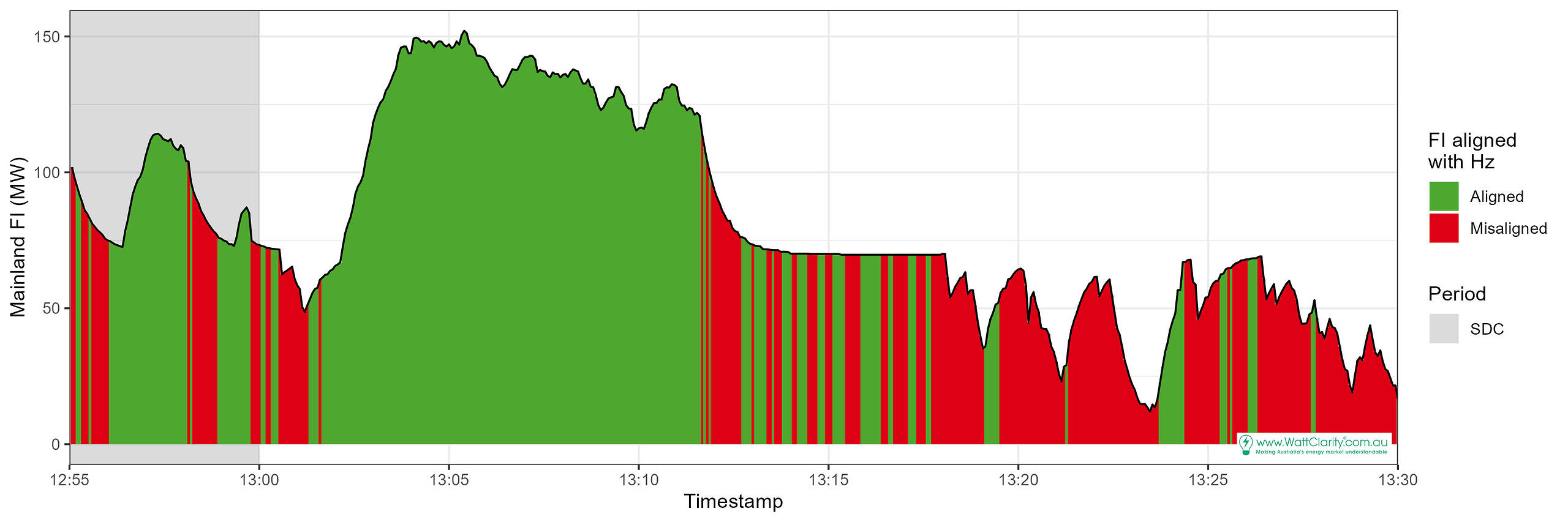
The FI in this example was consistently positive (chart below). Therefore, positive deviations (green ones in the chart above) would be evaluated as ‘helpful’. But only when the FI is aligned with the system frequency (Hz).

Deviations matching the need didn’t always earn a factor

The resultant 5-minute Causer Pays factors are not consistently ‘helpful’ where we’d ordinarily expect them to be. Deviations matched the need indicated by the FI in intervals from 13:10 to 13:30 but no factor was earned. The relevant 5-minute factors, for reference, are as follows.

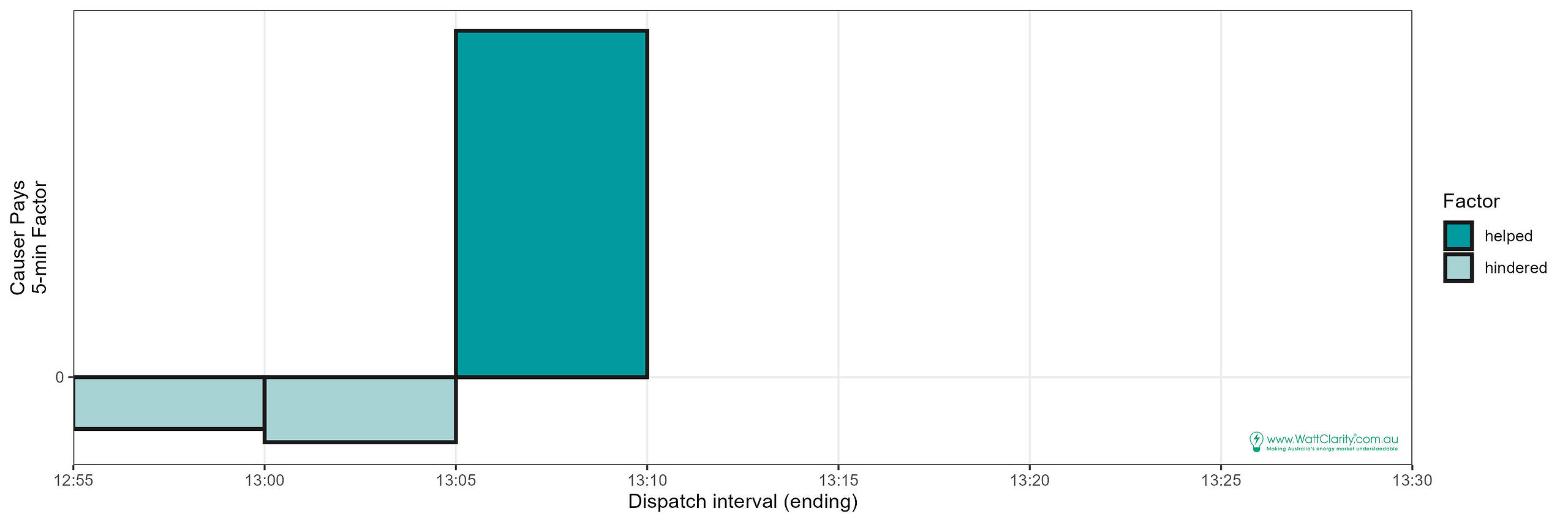
What happened in intervals 13:15 to 13:30?

Underlying reasons for the factor or lack thereof

There were two intervals judged unhelpful (hindered frequency). One interval helped. The remaining four intervals had no factors. To understand, we unpack each interval below.

FI alignment from the perspective of the unit’s deviations

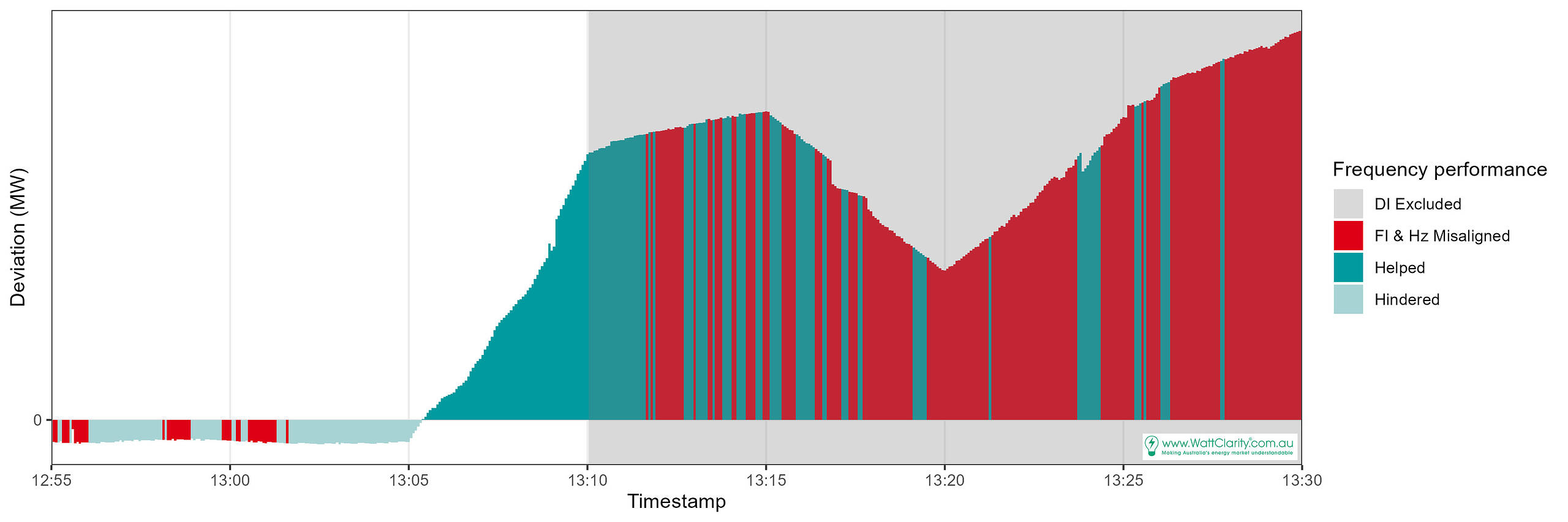
The final chart shows the 4-second unit deviations as they relate to the factors earned through the deemed contributions to frequency .

Each 4-second deviation gets a colour as to whether the FI was misaligned or, if not, how the aligned FI corresponded to the unit’s deviation (helped or hindered). Shading indicates excluded dispatch intervals. Red indicates excluded measurements.

The key takeaways

1. In this example only one of five biased intervals successfully earned a positive causer pays factor even though all five aligned with the indicator.
2. In these dispatch interval examples:
   1. Taking a guess at frequency to earn a positive causer-pays factor through self-forecast biasing appears at-best uncertain.
   2. The self-forecast bias might not produce a deviation that matches the FI (though in the 5 intervals here it did),
   3. The FI is often misaligned with system frequency, leading to exclusion of the dispatch interval (in two of the intervals here).
      1. The biasing effort produced no reward.
   4. Manual review of the data can lead to exclusion of the dispatch interval.
      1. Leading to the biasing effort producing no reward.

Going forward

On June 8 2025 the Causer Pays procedure to allocate Regulation FCAS costs ends and Frequency Performance Payments (FPP) replaces it.

That means the use of the FI for evaluating a unit’s contribution to system frequency is ending.

Consequently,  the sun is setting (has set, depending on when you read this) on this chapter of strategies that exploited the Frequency Indicator for regulation FCAS cost reductions.