As discussed in our previous note (Part 1) in this publication, ITK built a renewable NEM from scratch, aimed at meeting NEM-wide CY2025 demand. We focussed on generating a VRE portfolio with the highest Sharpe ratio, that is, the portfolio where average output could not be increased without also increasing variability. That study took no account of transmission.

In Part 2 below, we include an estimate of transmission but still require the portfolio to have VRE meeting a series of targeted “Sharpe” ratios; the ratio becoming a constraint, while the optimiser minimises cost. AEMO-modelled demand for CY2025 must be met in every half-hour period by the modelled VRE portfolio in combination with a fixed quantity of hydro (equal to historic NEM output), storage (pumped hydro, or more likely batteries) and variable quantity of gas. As hydro and storage output were fixed throughout the analysis, the quantity of gas power and gas generation are outputs of the model. A map of ITK’s preferred VRE portfolio – with the constraint Sharpe ratio ≥ 4 – is shown in Figure 1 below.

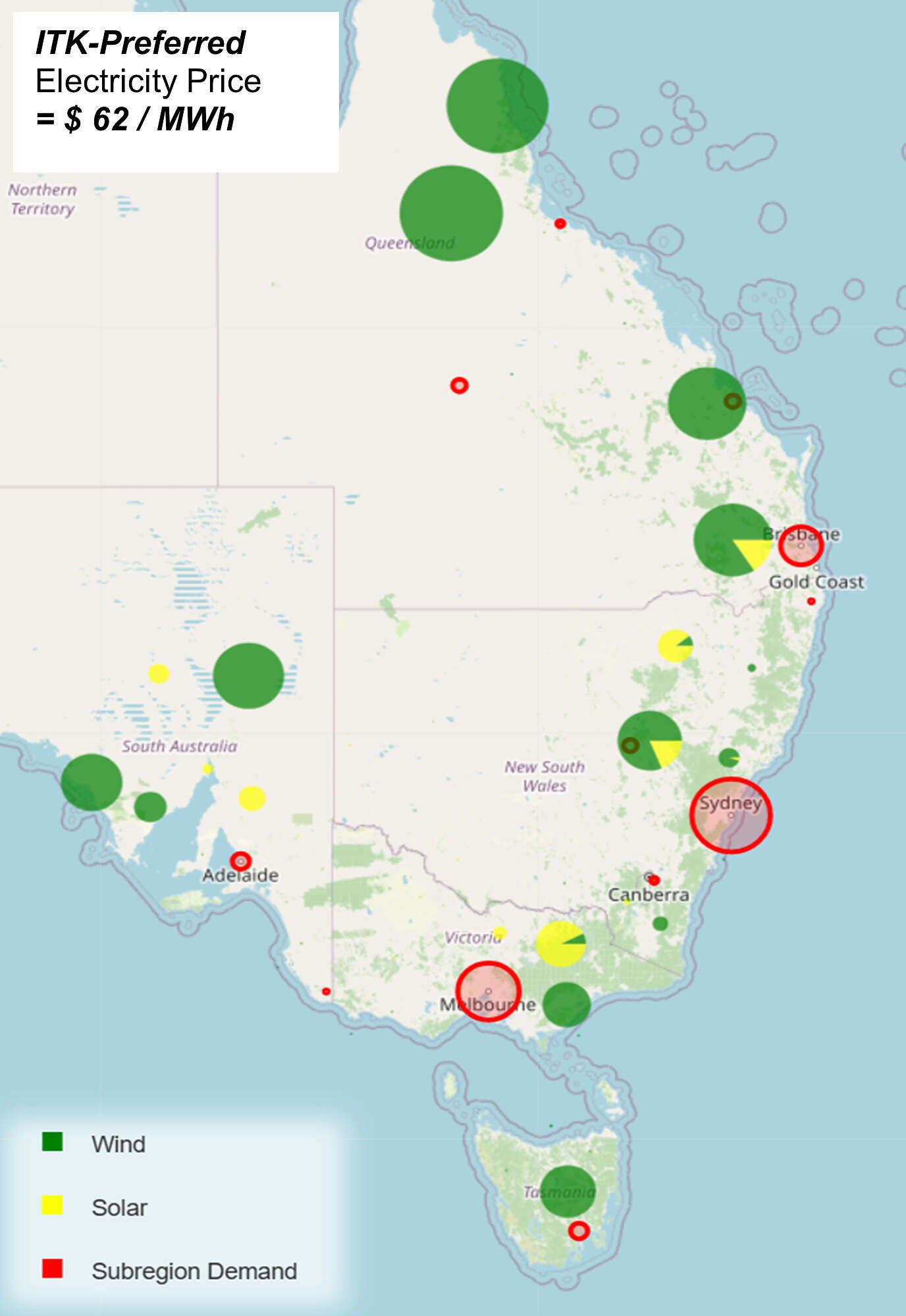
Figure 1: ITK Preferred VRE Portfolio Map

We use the portfolios generated to estimate the resulting electricity price that would provide a net present value (NPV) of zero in each case. Based on our (no doubt optimistic) cost assumptions, these prices turn out to be in the $60-$70 / MWh range, similar to that of consultants who looked at the NSW, Queensland and Victorian grid decarbonisation plans. If nothing else, this demonstrates that spending $200bn doesn’t result in a dramatic increase in electricity prices, quite the reverse. Eliminating most fuel and other variable costs leads to a stable and predictable price that is globally competitive. Our cost estimate does not include rooftop solar; it is taken as a “free good”. The authors learned a lot from this exercise, and we are grateful to AEMO for the data that makes such studies possible.

Key Findings

Based on the results from these desktop studies and subject to the numerous limitations discussed herein:

Targeting improved system reliability and reduced emissions drives the model towards greater reliance on wind, particularly situated at the fringes of the grid. This approach necessitates a more interconnected NEM and therefore increased initial investment in transmission networks but reduced firming costs in the long run.

The lowest cost solutions feature greater solar capacity, located closer to demand centres but extra firming gas to deal with resulting volatility. Figure 2 and Table 1 illustrate the two extremes, namely minimum cost over a short amortisation period and maximum system stability.

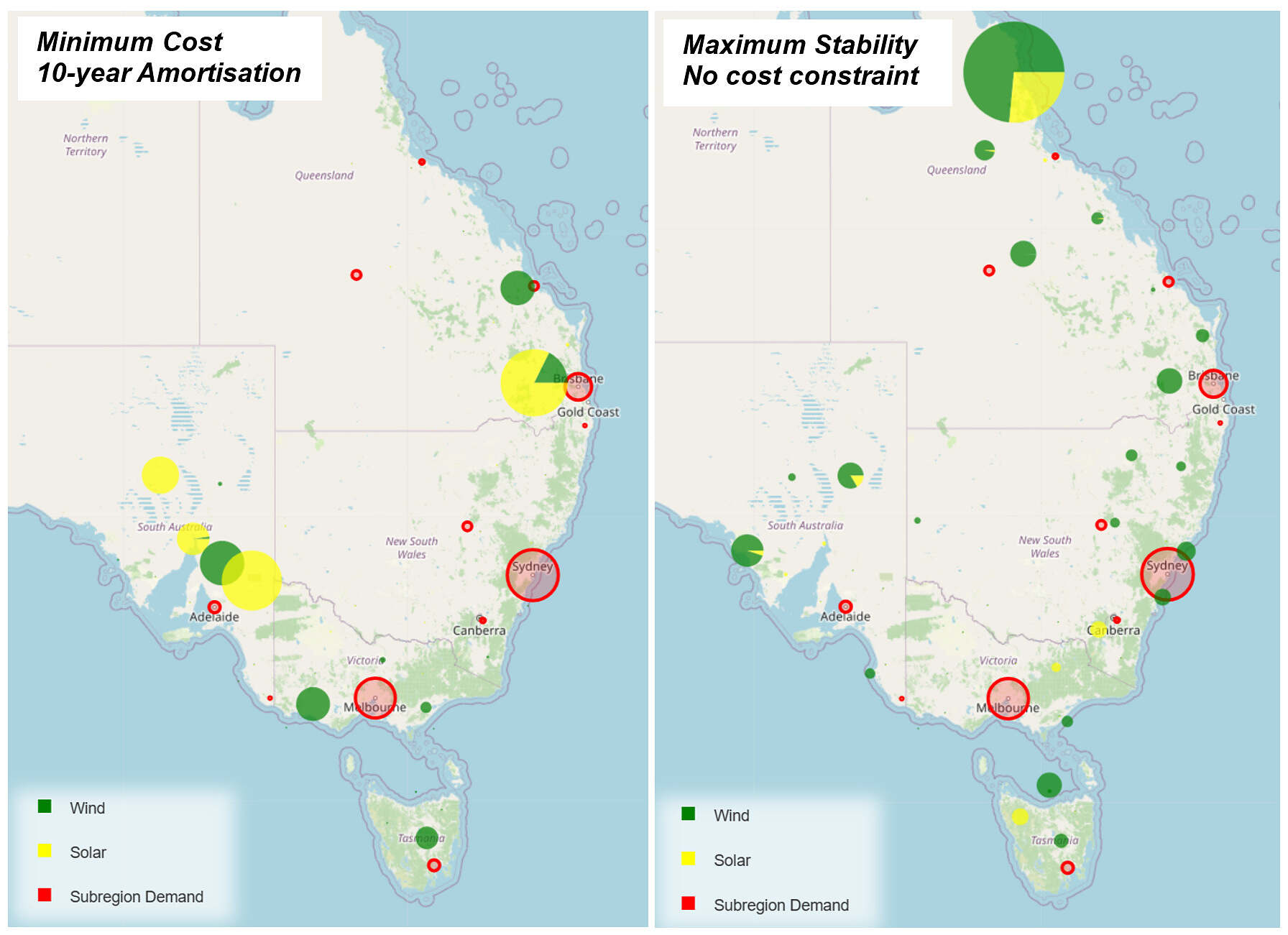
Figure 2: REZ Map for 10-Year Min-Cost (left) and Sharp-Optimized (right) VRE Portfolio

Table 1: System trade-offs
Minimum Cost / Short Amortisation	Maximum Stability / Long Amortisation
More solar, close to demand centres. Lower Transmission Network Costs Lower VRE Capital Lower VRE stability (Sharpe ratio) Higher Firming Requirements Higher Emissions Higher OPEX	More Wind, located towards fringes of grid. Higher Transmission Network Costs Higher VRE Capital Higher VRE stability (Sharpe ratio) Lower Firming Requirements Lower Emissions Lower OPEX

 

Amortising the system’s capital costs over longer periods yields similar results to increasing system reliability and reducing emissions. Namely, the compounding cost of fuel to supply firming gas plants over a longer period acts to disincentivise solar, driving greater reliance on wind energy especially at the fringes of the grid and, again, a more interconnected NEM. Figure 3 shows the Capital + 25-Year OPEX costs of systems modelled to minimize cost over 10-, 15-, 20-, and 25-year periods respectively.

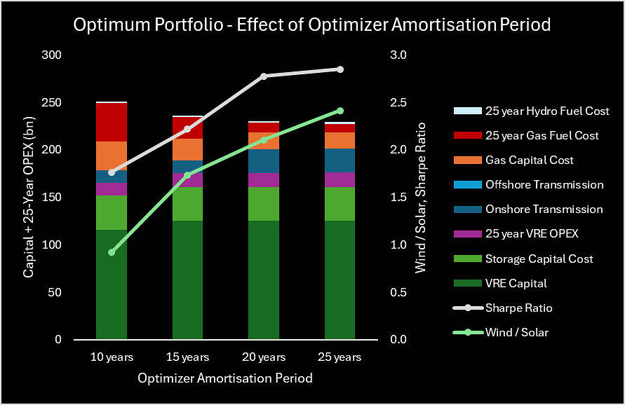
Figure 3: 25-Year Cost Breakdown for Portfolio Optimized at 10-, 15-, 20- & 25-Years Amortization[1]

With slightly higher upfront investment – compared to the lowest cost solution – we can significantly reduce carbon emissions and improve VRE portfolio stability by building a highly-interconnected system more heavily weighted towards quality wind assets at the fringes of the grid. To achieve this practically, ITK’s preferred VRE portfolio minimizes total system cost over 25 years subject to exceeding a minimum system reliability requirement (Sharpe ratio ≥ 4). See Figure 4 which shows cost breakdown for three key scenarios.

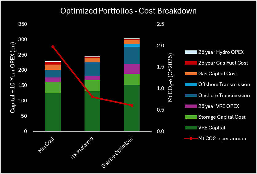
Figure 4: Cost Breakdown and Mt CO₂-e for: Min Cost, ITK Preferred, and Sharpe-Optimized Portfolios

In virtually all simulations and sensitivities, QLD ends up as a significant supplier of VRE and were it not for the higher costs of underwater DC transmission, TAS would also be favoured as a large exporter of wind. More wind in QLD – particularly in the Northern half of QLD – and more QLD/NSW interconnect capacity will be “low regrets” options in building out the low carbon NEM.

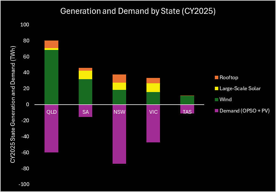
Figure 5: ITK Preferred Portfolio Generation and Demand[2] per State.

 

Method

Starting with a fresh sheet of paper, we build a wind and solar portfolio from AEMO’s renewable energy zones (REZ’s) – as detailed in the 2024 Draft Integrated System Plan (ISP) – add in existing behind the meter, and firm it with batteries, hydro, and gas to meet NEM-wide operational demand in every half-hour period for the calendar year 2025. We build multiple such systems using an optimization algorithm, each time varying the set of constraints/incentives given to the optimizer. The system constraints in each scenario are a combination of:

1. Volatility minimization – The Sharpe ratio of a portfolio is inversely proportional to its variability. Practically, we sought to maximise the stability of the VRE portfolio by increasing its Sharpe ratio.
2. Cost Minimization – Costs included:
   1. VRE Portfolio capital cost and fixed OPEX.
   2. Transmission Network capital cost.
   3. Storage capital cost.
   4. Firming Gas capital cost and running fuel cost.
   5. Hydro OPEX.
3. TAS Generation limit – When stated, we assume that Tasmanian generation surplus to state demand must be transmitted to Victoria, therefore incurs DC transmission costs.
4. REZ generation limits – Capacity of wind and solar for each REZ are set to the “Renewable Potential (MW)” values stated in AEMO’s 2024 Draft ISP.
5. VRE Portfolio generation – represented as the ratio VRE Portfolio Gen / NEM CY25 Demand. Sensitivity analysis shows that ~100% – 110% of NEM CY25 demand is ideal.
6. Years’ OPEX included in total system cost.

Battery power and storage are fixed at 15 GW and 4 hours. Hydro power and capacity are fixed at 7.5 GW and 14 TWh. These values could be optimized in future simulations, as we know that for any given VRE portfolio, more battery/hydro means less gas and vice versa.

Firming / Seasonality

A VRE portfolio with annual output equal to or greater than demand in the NEM inevitably requires “firming” supplied by some combination of storage, hydro and gas. In designing such a system there are various trade-offs between transmission and firming costs. Systems built to minimize the total firming requirement will end up with more wind, much of which will be located around the perimeter of the grid, and therefore result in greater transmission requirements. Once transmission costs are allowed for, a lower overall cost solution is to have more solar located closer to demand, and to handle the resulting volatility with extra firming using gas.

A feature of a high VRE grid is strong seasonality. Output from solar is lower in winter and wind is also seasonal. When only batteries or pumped hydro are used to deal with wind and solar supply shortfalls our work shows that, for any “reasonable” quantity of storage, it is often empty. This is particularly the case in winter. Our analysis shows that using gas earlier in the merit order during winter resulted in lower requirement for storage capacity while retaining “low” gas consumption. By contrast, using storage early in the supply sequence during spring and summer – when VRE output tends to exceed demand – minimises the use of gas.

We note that once again QLD output helps with seasonality droughts, as QLD wind tends to be better in Winter and less in Summer.

Sharpe Ratio

The Sharpe ratio of a portfolio is inversely proportional to its variability. Average output of the Sharpe ratio-maximised portfolio cannot be increased without incurring more volatility.  Practically, we first maximised the stability of the VRE portfolio by increasing its Sharpe ratio. This showed that the highest Sharpe ratio portfolio was dominated by Qld and Tasmania onshore wind, but also included about 19% solar and a small amount of offshore wind. A major limitation of this analysis being the omission of transmission costs.

Subsequently we estimate the cost[3] of the system (capital costs, transmission network costs and OPEX) and generate several cost-minimised portfolios, gradually introducing minimum Sharpe ratio constraints. Increasing the minimum Sharpe ratio requirement of the cost-optimizer incentivises widening the geographical distribution of power generation, i.e., more generation near the fringes of the grid. This is intuitive: generally, the greater the distance between two REZ’s the less correlation there is between the weather conditions at the two locations, particularly for wind. This effect is clearly observed in the correlation matrices of the wind and solar capacity factors (Figure 6 and Figure 7).

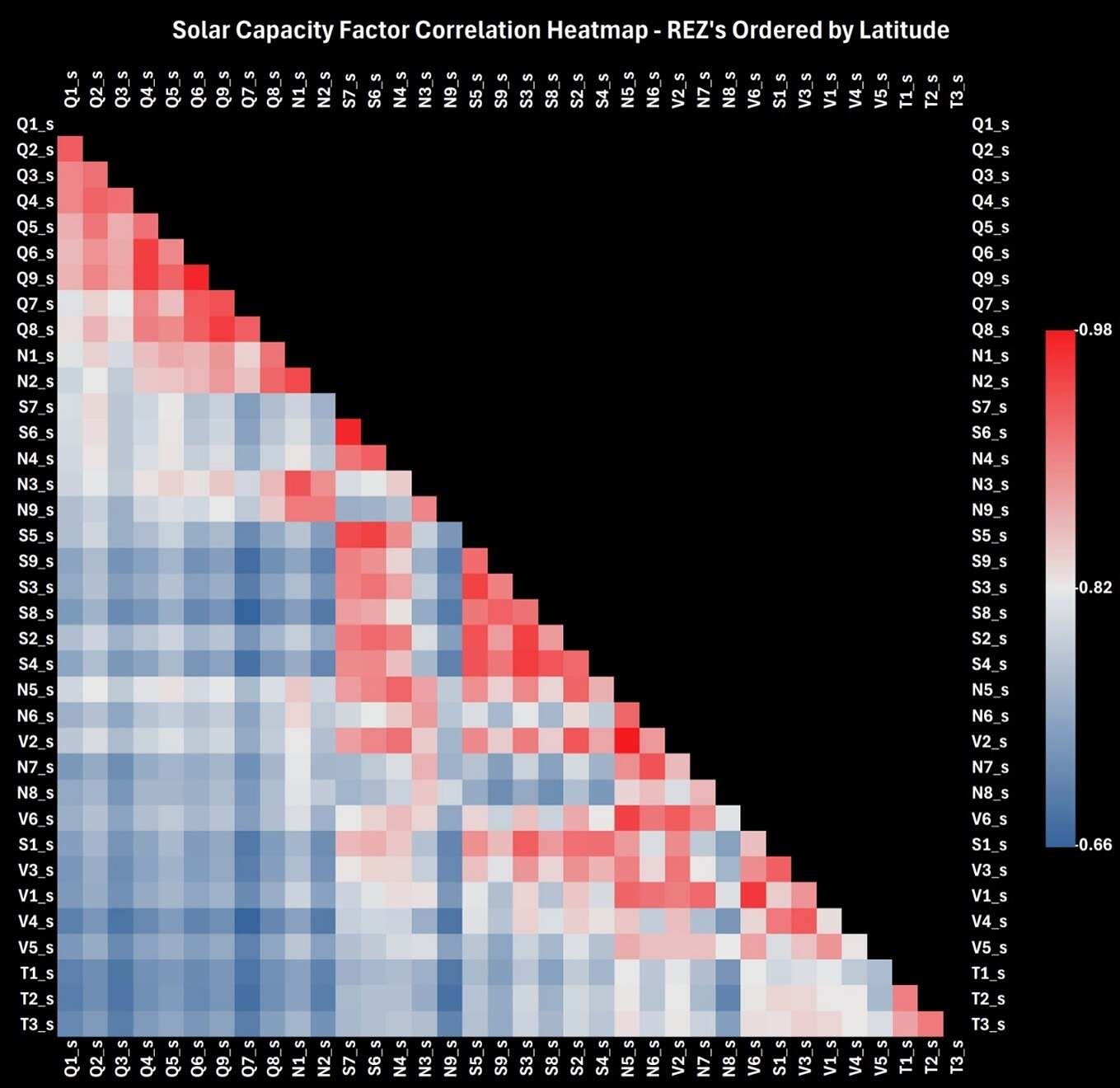
Figure 6: REZ Solar Capacity Factor Correlation Matrix – Ordered by Latitude

 

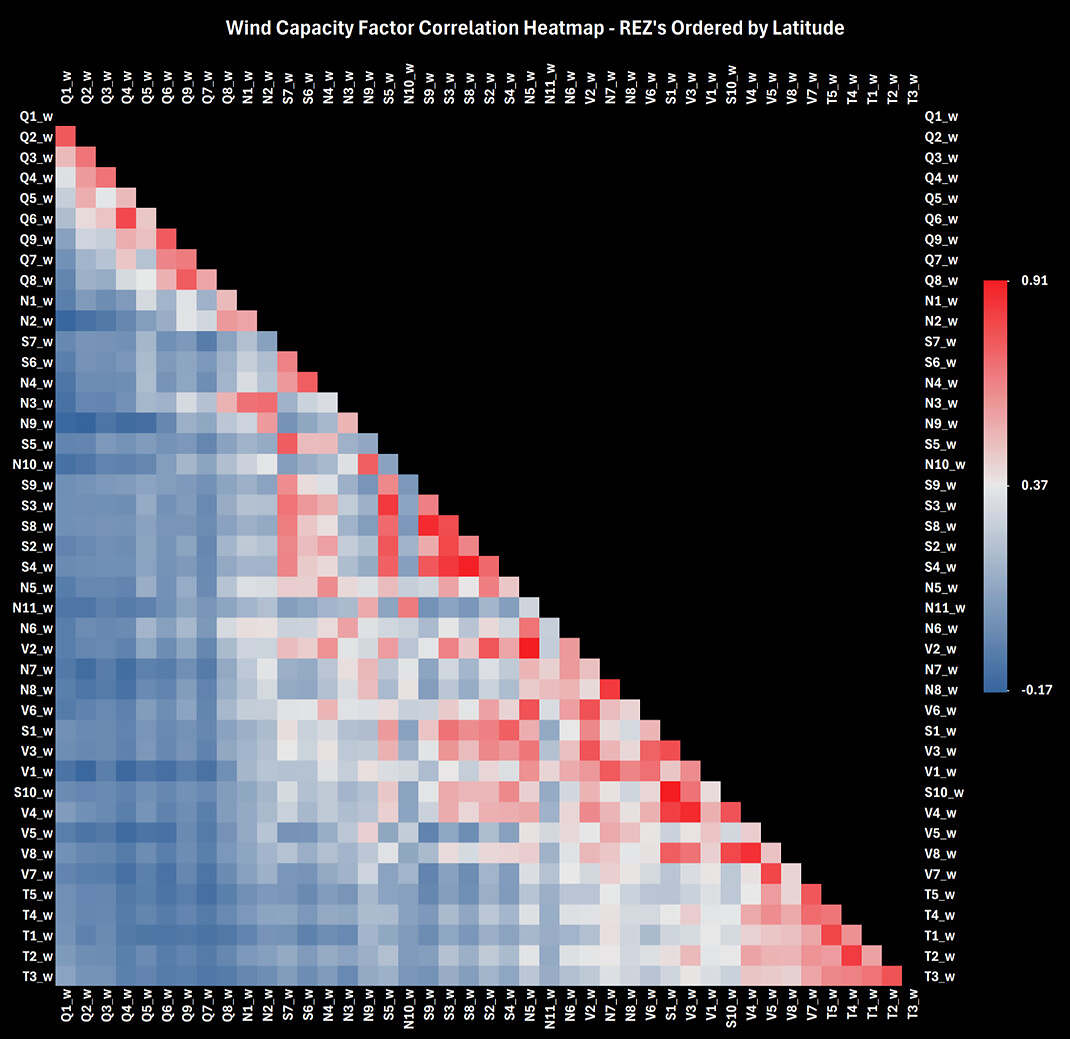
Figure 7: REZ Wind Capacity Factor Correlation Matrix – Ordered by Latitude

In a Sharpe-optimised system, there is a lot of incentive to allocate weight to REZ’s in Northern Queensland (farthest North), Central South Australia (farthest West) and Tasmania (farthest South) as this achieves the widest possible geographic spread of generation. We see this assertion supported in Figure 2.

Increasing the Sharpe ratio also incentivises wind – particularly Tas and Qld wind – over solar, again intuitively, because:

• the power generation of a higher-Sharpe-ratio portfolio would drop less drastically overnight.
• Solar capacity factors from separate REZ’s have a much stronger correlation with each other than wind capacity factors. Increasing wind in the portfolio therefore has a greater upwards influence on Sharpe ratio than solar. See Table 2. The Sharpe ratio of an evenly weighted solar-only portfolio is about a third of the Sharpe ratio of an evenly weighted wind-only portfolio.

Table 2: Sharpe Ratio for Solar and Wind Only Portfolios
Portfolio	Sharpe Ratio
Solar Only (Evenly Weighted)	0.83
Wind Only (Evenly Weighted)	2.52
Sources: AEMO Draft 2024 ISP

As such, as we increase the minimum acceptable Sharpe ratio (model constraint) in our cost minimisation model we observe:

1. More generation at the fringes of the grid, therefore higher onshore transmission cost.
2. VRE portfolio weight more heavily allocated to wind.
3. Lower firming requirements – and therefore lower gas capital and fuel costs – as the more stable portfolio with higher wind meets NEM demand in a greater portion of half-hour periods. This has an exaggerated effect on the system balance through peak demand, and overnight, as solar trails off.

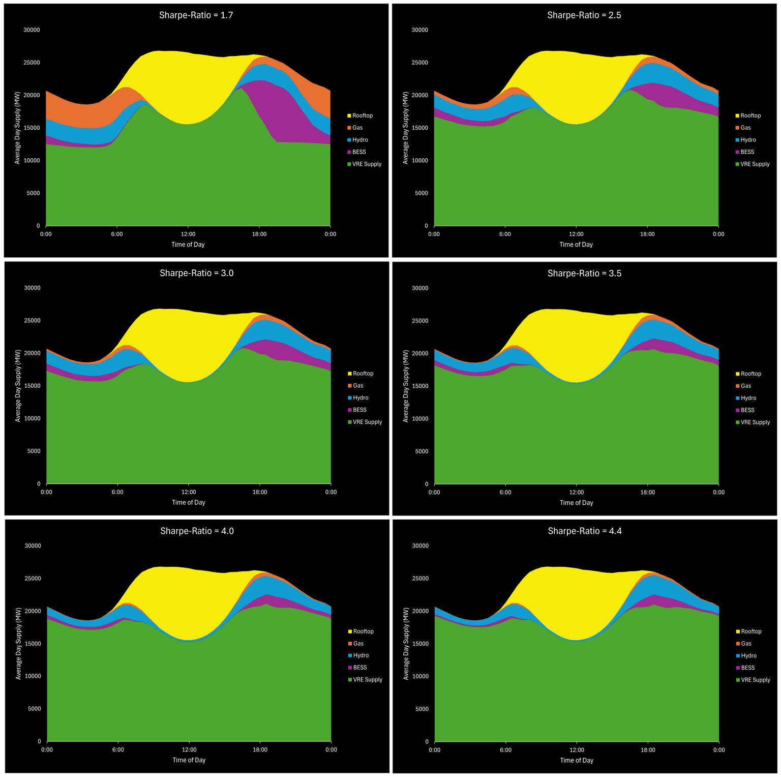
Figure 8 illustrates the effect of increasing the Sharpe ratio on the average day power supply by source (i.e., more VRE, less firming).

 

Figure 8: Average Day Supply by Source at Different Sharpe Ratios. Click here to see a higher-resolution version.

 

VRE Portfolio Scale – Effect on Cost

As VRE Portfolio capacity relative to NEM demand (“VRE Scale” hereon) increases, system capital cost increases but firming capacity requirements decrease. To minimise long-term costs, VRE portfolio generation should be set to 100-110% of CY2025 demand. See Figure 9, which models the costs of ITK’s preferred portfolio at various values of VRE Scale. The optimal setpoint for this ratio achieves the best trade-off between VRE capital costs and gas fuel costs. Although slightly more costly, 110% VRE Scale was preferred, because it had substantially lower gas requirements than 100%.

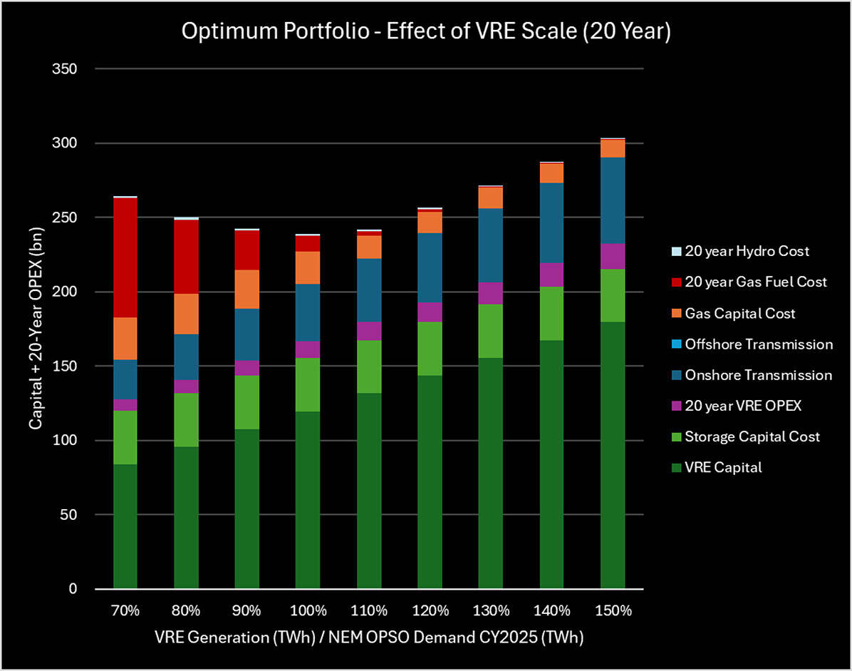
Figure 9: Effect of “VRE Scale” on System Cost and OPEX

 

Solar % of VRE Portfolio

A similar sensitivity analysis was conducted on the Wind / Solar ratio, by varying the relative amount of each within the portfolio (retaining REZ ratios within each generation type). The optimum mix sits at around 18.5% Solar (using Draft ISP 2024 data). The greater the solar, the lower the capital cost, but this comes at the expense of significantly higher firming requirements, and therefore higher long-term cost.

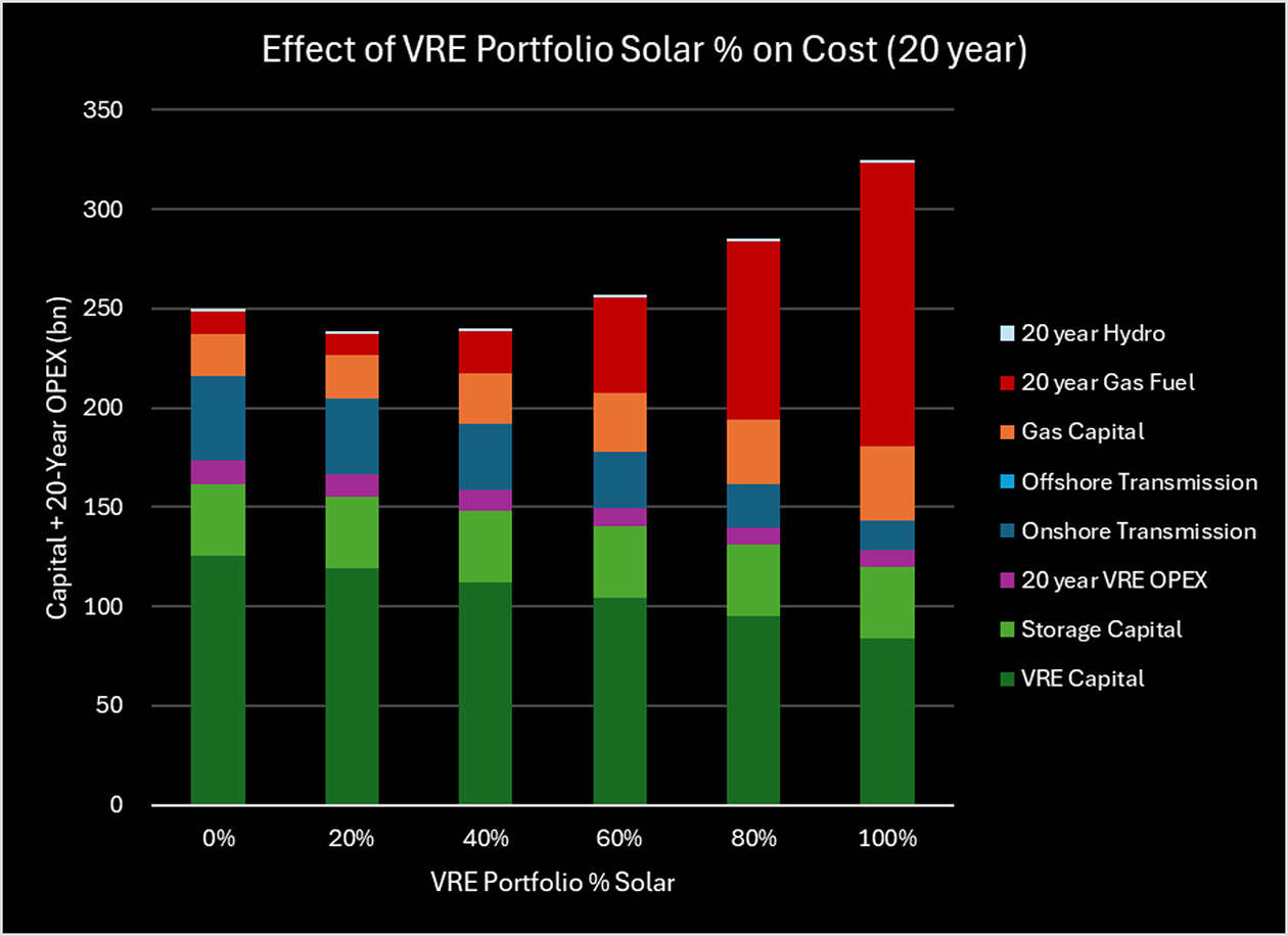
Figure 10: Effect of VRE Portfolio % Solar on System Cost and OPEX

 

ITK-Preferred Portfolio

ITK prefers a slightly more expensive system (than the absolute minimum cost) with greater transmission requirements but significantly lower reliance on gas. This portfolio minimizes the 25-year total cost of the system with the following additional requirements:

1. a Sharpe ratio ≥0 (set as a constraint in the optimisation model)
2. VRE scaled to generate 110% of NEM total demand in CY2025, and
3. Tas generation surplus to state demand must be transmitted to Victoria, therefore incurs offshore transmission costs. Given the high cost of DC transmission, this constraint renders Tas generation surplus to state demand nonviable.

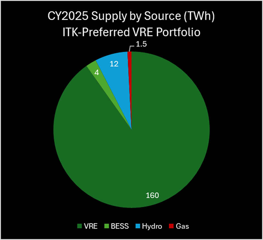
Figure 11: ITK-Preferred VRE Portfolio Supply by Source

ITK’s preferred portfolio consists of:

2025. 58 GW of VRE supplying 160 TWh in CY2025.
2026. 15 GW / 4h of BESS supplying 8 TWh in CY2025.
2027. 13 GW of firming gas supplying 5 TWh in CY2025.
2028. 5 GW / 14 TWh of Hydro supplying 12 TWh in CY2025.

Costs

In this note, costs are not intended to be indicative of actual costs but rather are goals set in the optimisation function. Specifically, the optimiser takes no account of existing assets other than hydro. No account is taken of existing gas, existing wind and solar or existing transmission.

Equally because the VRE and storage are built on an “overnight” basis, no allowance is made for learning rate impacts which are expected to drive down the costs of solar and batteries, particularly over the next decade. ITK’s personal expectation is that once we get into the transmission building phase of the transition that some improvement in the cost outlook for this component can be achieved.

That said the unit costs and weights of three systems that we built are shown in Table 3:

1. Lowest cost portfolio, 25-year total cost minimised, Tas generation constrained[4]
2. ITK’s preferred portfolio, 25-year total cost minimised, Tas generation constrained, VRE portfolio Sharpe Ratio ≥
3. Sharpe-optimised portfolio. No cost constraint, Sharpe ratio maximised.

Table 3: REZ Optimisation Portfolio Comparison
		Lowest Cost	ITK Preferred	Sharpe- Optimised
Sharpe Ratio		2.8	4.0	4.4
CO2-e (Mt / annum)[5]		2.0	0.8	0.6
Cost (bn)
VRE Capital		125	131	152
Storage Capital Cost		36	36	36
Onshore Transmission		25	43	57
Offshore Transmission		0	0	8
25-year VRE OPEX		15	15	31
Gas Capital Cost		17	15	15
25-year Gas Fuel Cost		9	4	3
Capital + 25-yr OPEX		229	246	303
Weight Allocated
NSW	Solar	2%	4%	4%
QLD	Solar	10%	2%	7%
SA	Solar	17%	7%	2%
TAS	Solar	0%	0%	4%
VIC	Solar	0%	6%	2%
NSW	Wind	7%	8%	15%
QLD	Wind	28%	39%	39%
SA	Wind	16%	18%	15%
TAS	Wind	6%	6%	9%
VIC	Wind	13%	9%	2%
Total	Solar	29%	19%	19%
Total	Wind	71%	81%	81%

 

Table 4 details our cost input assumptions.

Table 4: Cost Inputs
Item	Unit Cost ($)	Unit
Gas Capital	1,200,000	/ MW
Solar Capital	1,200,000	/ MW
Onshore Wind Capital	2,500,000	/ MW
Offshore Wind Capital	4,500,000	/ MW
Storage Capital	600,000	/ MWh
Gas Fuel	100	/ MWh
Storage Dispatch	–	/ MWh
Hydro Dispatch	5	/ MWh
Onshore Transmission	2,000	/ MW / km
Offshore Transmission	15,000	/ MW / km

To find the price of electricity required to justify the investment, we ran an NPV analysis and set the price at a level which ensures an internal rate of return (IRR) equal to the weighted average cost of capital (WACC). This required all assets, both new and existing, to earn a return on capital and recover all OPEX.

A shortcut to this process is to take our capital costs per Table 4, add in a cost of $3m / MW for 7500 MW of existing hydro, and also allow $12 / MWh for wind and $5 / MWh for solar OPEX, solely for this specific levelized cost objective. This analysis yielded the following required electricity prices:

Table 5: Required Electricity Prices for Modelled VRE Systems
VRE/Firming System	Required Electricity Price
Lowest Cost	$ 58 / MWh
ITK Preferred	$ 62 / MWh
Sharpe-Optimized	$ 70 / MWh

From another point of view, one could look at the change in the quantity of gas generation under each of the scenarios, convert that to gas consumption and then calculate the marginal cost of CO₂ abatement as (change in system costs / change in CO₂).

Conclusion

• More solar means lower stability and more firming requirements but is cheaper. A cost-minimized system with no other constraints favours solar, closer to demand centres. If the amortisation period is increased, compounding firming gas fuel costs drive the balance towards wind.
• As we increase Sharpe ratio minimum constraints, we see solar gradually dropped for wind, and long-term gas costs traded off for upfront transmission costs.
• A Sharpe-maximized (high stability) system more heavily favours wind, particularly at the fringes of the grid, in REZ’s with higher quality renewable energy leading to lower system volatility and firming costs/emissions but higher transmission costs.
• The high modelled cost of offshore wind means that none of the cost-minimised systems allocate weight to offshore wind REZ’s.
• ITK’s preference is a highly interconnected, wind-heavy, stable, and low-carbon NEM. Practically this is achieved by generating a 25-year cost-minimized portfolio with a minimum Sharpe ratio requirement.

Limitations

• Round-trip efficiency losses are ignored.
• The transmission system modelled is rudimentary. Further work could model the transmission network and associated costs more accurately and ensure that demand at each of the sub-regional demand centres was appropriately met.
• Firming dispatch order is (essentially) fixed, aside from a simple order change in summer/spring vs. winter/autumn. Future work could model a dynamic dispatch order.
• Battery and hydro capacity were fixed. Both the power and hours available components of storage and hydro could be optimized in further simulations.
• System costs are rudimentary and do not include rooftop, which is taken as a “free good”.

 

[1] The optimiser is programmed to generate the lowest cost portfolio over 10, 15, 20 and 25 years respectively. The cost breakdown indicated is the 25-year total system cost for each of these portfolios.

[2] Demand values shown below the x-axis (negative)

[3] In this note costs are not intended to be indicative of actual costs but rather goals set in the optimisation function

[4] Tas generation above state demand incurs offshore transmission costs, as it must be transmitted to Victoria.

[5] CO₂ equivalent emissions from firming gas supply, assuming 1 MWh gas = 0.54 Mt CO₂-e

---

About our Guest Authors

 

---