
As we were reminded (several times) in AEMO’s 2024 Draft Integrated System Plan (ISP), “Renewable energy connected by transmission, firmed with storage and backed up by gas is the lowest cost way to supply electricity to homes and businesses throughout Australia’s transition to a net zero economy”.
In light of AEMO’s assertion, starting with a fresh sheet of paper we built a maximum Sharpe ratio wind and solar portfolio, added in existing behind the meter and firmed it with batteries, hydro and gas to meet NEM-wide operational demand for the calendar year 2025. Professor William Sharpe won a Nobel prize in 1990 for his contributions to the Capital Asset Pricing Model (CAPM) in finance and also developed the so-called Sharpe Ratio. The key insights of Sharpe and his colleagues was to show that a portfolio of shares would have a lower variability for a given return than any individual stock. A corollary is that it’s the contribution of the stock to the portfolio that matters rather than the merits of the stock in isolation. It seemed to us that these concepts were applicable to wind and solar. A portfolio of wind and solar farms will have a lower variation for a given capacity factor than individual projects. The Sharpe ratio for wind and solar projects is operationalised as the expected capacity factor/divided by standard deviation.
Using Python and an optimiser and AEMO half-hourly REZ traces for wind and solar we built a 1 MW maximum Sharpe ratio portfolio and then using AEMO half hourly demand forecasts scaled the portfolio so that total demand equalled total supply. Then we calculated sequential half hourly demand and supply balance resulting in either energy available for storage or firming required. Enough firming was provided so that demand was met in every half hour for CY 2025. We then applied capital costs, and in the case of gas fuel costs, to build up the total cost of the system and then ran sensitivity tests with the objective of minimising total system cost. Our work remains at an early stage, even though in Leitch’s case he’s been developing this concept for more than four years. A glaring, but soon to be remedied element of this thought experiment is that transmission costs are not yet included. Once they are we expect the optimal solution to change. To the extent this work has any value it’s in comparing what a theoretical new system might look like with the existing system. Above all the exercise shows the benefit of diversification of renewable resource but, because of transmission, the cost of achieving it. Another epiphany is that optimisation in the use of storage assets can greatly reduce the overall cost.
As part of the work, we take advantage of new data provided with the ISP 2024 data set such as sub-regional demand, and also briefly compare the 2024 ISP demand forecast with that of 2022.
Key Takeaways
- Industry lore of 75% wind / 25% solar holds (almost) true in our VRE portfolio optimisation exercise. We incentivised a model to generate a solar/wind portfolio from AEMO’s Renewable Energy Zones (REZ’s) that maximizes its return relative to risk (Sharpe ratio), and no constraints were placed on the proportion of wind and solar, nor the geographical distribution of the generation. The generated portfolio came to 77% wind, 23% solar. Indeed, in subsequent sensitivity analyses, varying the wind to solar ratio either side of this optimum increased the long-term costs of the system (capital + fuel + firming dispatch). Increasing solar % of the portfolio decreases the upfront costs, but significantly increases firming capacity requirements and expenditure on fuel for firming gas generation over time.
- Generation in this Sharpe-ratio optimsed portfolio is very heavily weighted to Far North Queensland. This portfolio sees Qld, SA, and Tas being net exporters, NSW and Vic net importers of energy. Given the location of the demand centres, it is highly likely that an optimised system which accounts for transmission costs will shift generation further South.
- The optimised VRE + Firming Capacity system modelled in this analysis requires:
- 56 GW of Variable Renewable Energy capacity supplying 160 TWh of energy in 2025,
- 15 GW / 4 hours of storage capacity supplying 3 TWh of energy in 2025,
- 5 GW / 14TWh of (existing) Hydro, and
- 8 GW of open cycle gas supplying 4 TWh of energy in 2025.
The total capital (excluding Hydro) is $169 billion. The VRE cost is $123 billion, and gas firming capacity cost $46 billion.
- The amount of battery storage required is dependent on the order in which firming resources are used. If Batteries are dispatched first the seasonal nature of VRE production means that there will be large surpluses at times but also very large deficits. If dispatched last the batteries spend too much time at full capacity with surplus VRE wasted. Realistically there is a large incentive to discharge full batteries when sunlight is abundant. By dispatching batteries first in Summer but last in winter, an additional 6 TWh of additional energy can be supplied by batteries instead of gas. Refining the dispatch algorithm seems to offer the promise of further reducing the overall theoretical cost.
2022 ISP vs. 2024 ISP
The 2024 ISP generally forecasts higher rooftop PV compared with the 2022 ISP. This gap starts relatively small (around 2023-2025) and significantly widens over time. According to the AEMO 2024 Draft ISP “Consumer Energy Sources are forecasted to be taken up even faster than before, with 18GW more rooftop solar by 2050 under Step Change compared to the 2022 ISP”. Increased EV uptake also significantly bumps daytime total demand, as consumers leverage increased rooftop solar to charge their cars.
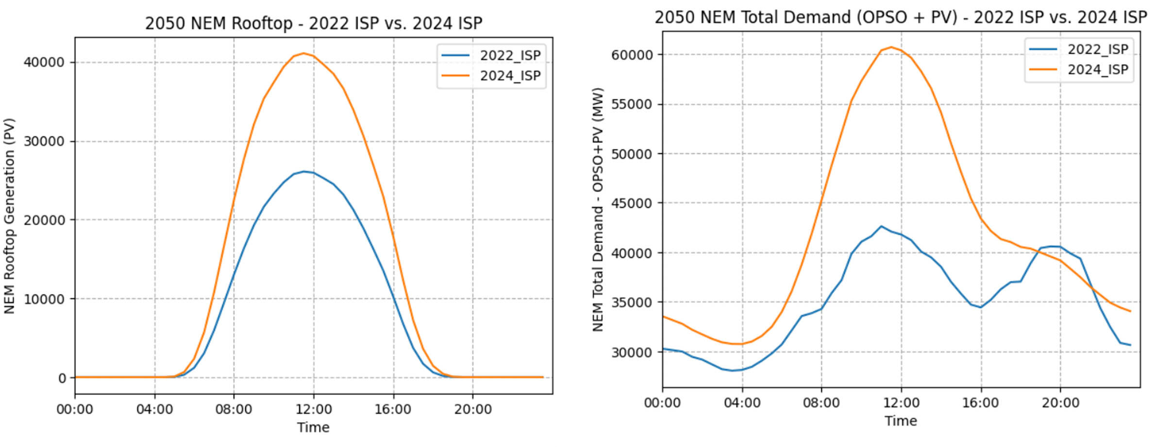
Figure 1 – 2024 ISP demand forecast compared to 2022 forecast by time of day in 2050 (Source: AEMO 2022 ISP and 2024 Draft ISP)
Sharpe-Ratio-Optimised VRE Portfolio
Sharpe Ratio and Portfolio Diversification
Using 2022 ISP wind and solar half hourly traces from 2023/07/01 – 2052/06/30 (508464 datapoints) we generated a VRE portfolio that maximizes return (mean REZ capacity factor) relative to risk (standard deviation of REZ capacity factors). In other words, weights are distributed across the REZ’s in order to maximize the portfolio’s Sharpe ratio. While our optimiser doesn’t impose geographical distribution constraints, the Sharpe ratio inherently encourages diversification across REZ’s by forcing it to reduce portfolio volatility. For instance, when wind is subdued in Far North Queensland (Q1), it may be blowing a gale in Tasmania, but probably not in the North Qld Clean Energy Hub (Q2). Indeed, a 50% Q1 wind / 50% Q2 wind portfolio has a lower Sharpe ratio than 50% Q1 wind / 50% T1 wind (0.95 compared to 1.03), to provide a very simple example. For the same reason, the Sharpe ratio incentivises a mix of solar and wind – the wind still blows while the sun doesn’t shine – even though wind on average has a much higher average capacity factor than solar.
Result
Figure 2 shows how the Sharpe-ratio optimised portfolio is distributed across the states and between solar and wind. It is heavily weighted to Far North Queensland (REZ Q1), with 12.2% of the entire portfolio in Q1 wind and 5.4% in Q1 solar. Figure 7 illustrates how the weights are distributed across the REZ’s. Conceptually, the optimisation algorithm has sought out a high capacity-factor wind REZ and heavily weighted towards that, while still allocating the rest of its weight relatively evenly across the country. Also note that the Queensland REZ’s are spread over a wider range of latitudes than the REZ’s in other states. The portfolio sees Queensland as by far the biggest generator and has a wind to solar ratio that is line with industry lore, 77% wind, 23% solar (lore ~ 75, 25).
It’s worth noting that during a quick VRE portfolio cost minimization exercise – algorithm was incentivised to minimize total capital cost of VRE portfolio – with the constraints (1) NEM OPSO demand is met and (2) a minimum Sharpe ratio was exceeded: Q1 was weighted even more heavily (> 30% of total portfolio). Again, this makes sense conceptually. As we reduce the incentive of the optimiser to increase the Sharpe ratio, its incentive to diversify the portfolio diminishes, leading to a greater emphasis on high-capacity-factor REZ’s. In this case, the algorithm cares more about maximizing capacity factors and minimizing cost / MW of generation than it does maximizing the stability of the system.
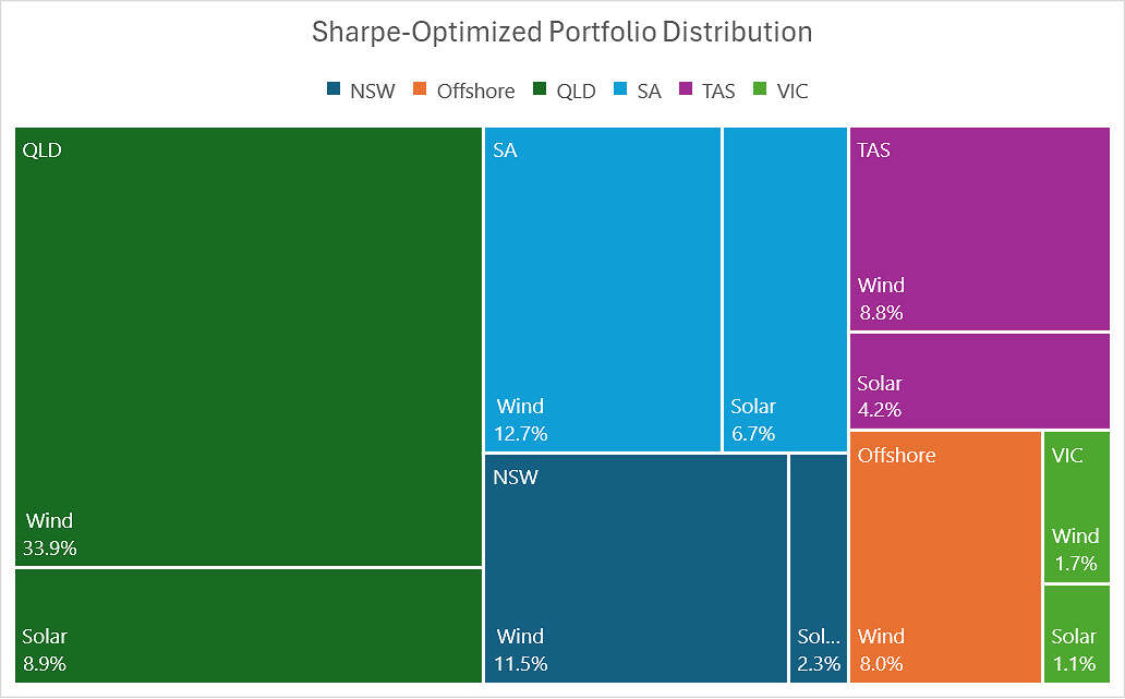
Figure 2 – Tree map of Sharpe-Ratio Optimised Portfolio Distribution
State Demand vs. Generation
Queensland, SA, and Tasmania will be net exporters and Victoria and New South Wales net importers of energy based on our VRE portfolio and 2025 operational demand. The net importers happen to be the states with densest population, by a significant margin, see Figure 3. Logically, this net import/export status is partially explained by having less land available for high quality renewable energy generation per (energy-consuming)-capita in the densely populated states.
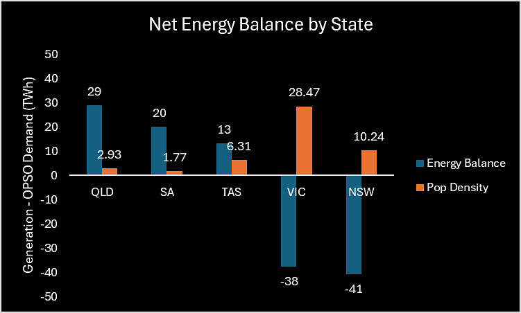
Figure 3 – Net Energy Balance and Population Density by State 2025 (Source: AEMO 2022 ISP)
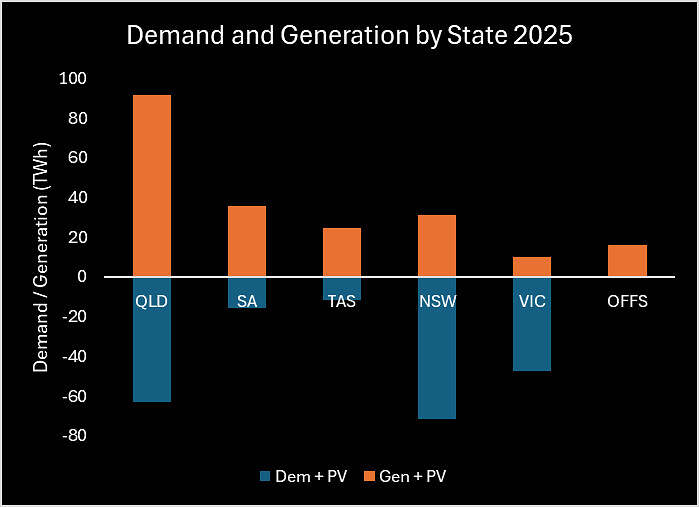
Figure 4 – Demand and Generation by State 2025 (Source: AEMO 2022 ISP)
It is also explained by the quality of renewable energy in each of the states. Vic and NSW’s REZ’s have the lowest mean capacity factors, highest CFs are in Tasmania and Queensland. Figure 5.
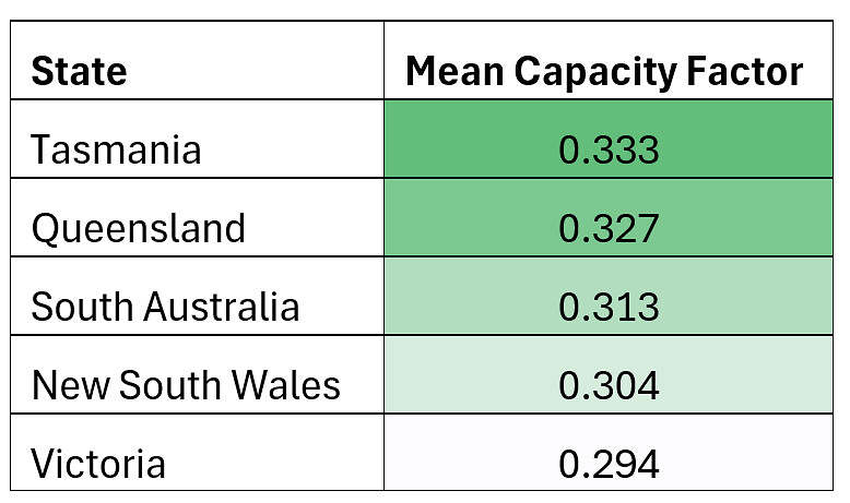 Figure 5 – State average Renewable Energy Capacity Factors (Source: AEMO 2022 ISP)
Sub-Regional Demand
Figure 6 shows how heavily NEM demand is weighted towards the NEM’s lower latitudes (Sydney-Newcastle-Wollongong and Victoria subregions alone make up > 50% of NEM demand in 2025).
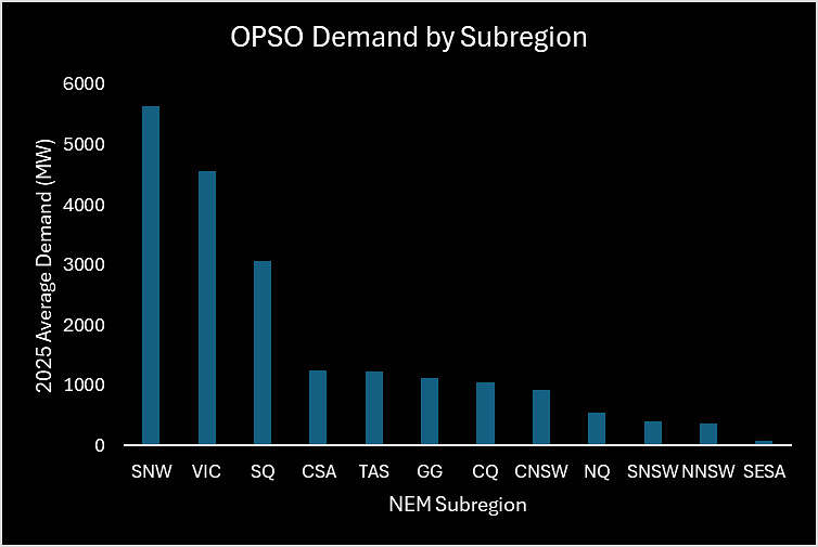
Figure 6 – 2025 OPSO Demand by NEM Subregion (Source: AEMO 2024 Draft ISP)
To contextualize the distance between our VRE portfolio generation and demand centres, Figure 7 illustrates demand by sub-region alongside VRE portfolio generation on an Australian map. The significant distance between the highest-generating REZ’s and the highest-demand sub-regions underscores the need to incorporate associated transmission costs in future iterations of portfolio optimisation. Given the considerable distance of the Far North Queensland REZ from major demand centers, transmission costs are likely to redirect a lot of this energy generation further South.
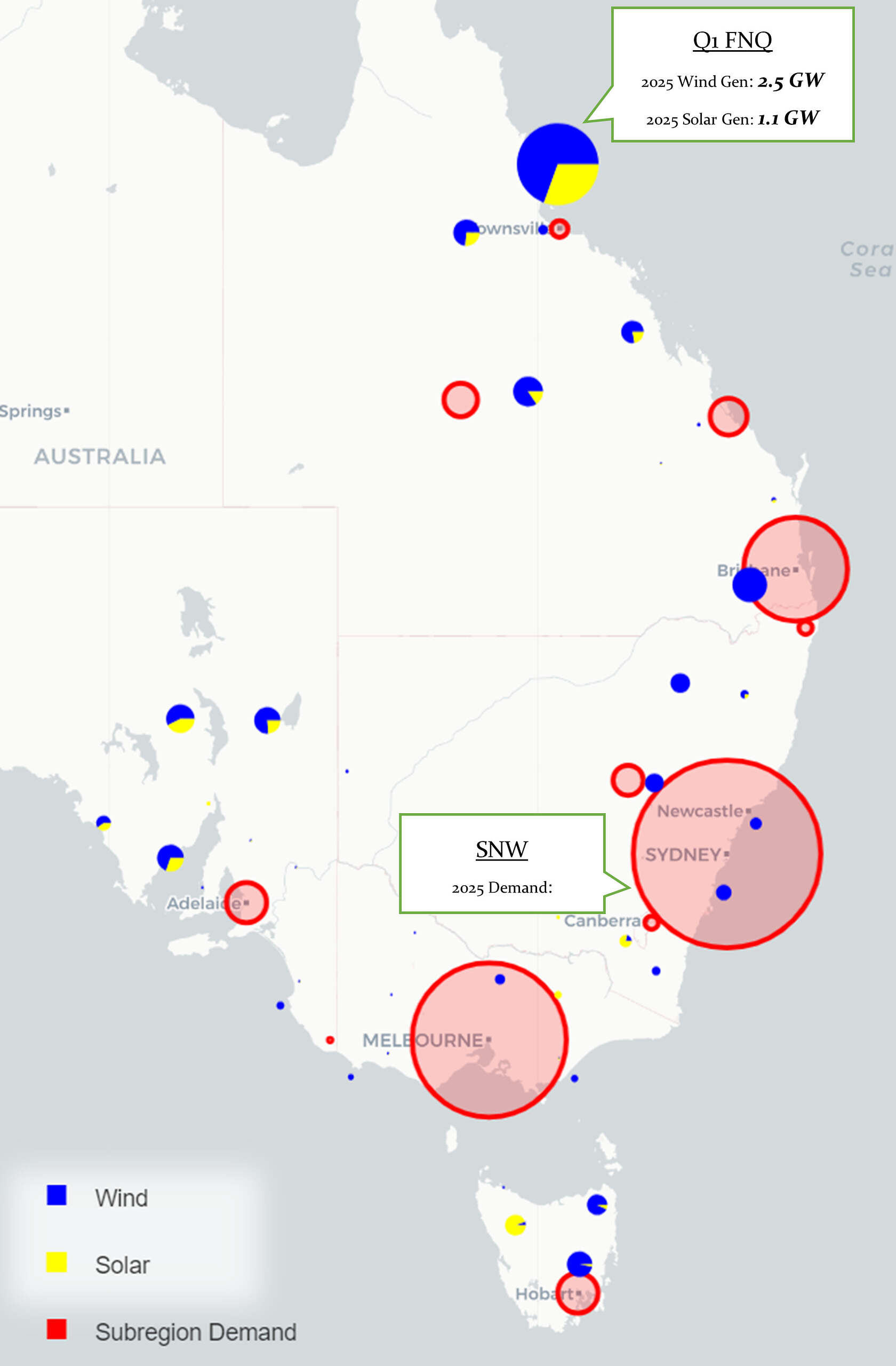
Figure 7 – Sharpe-Optimized Portfolio Generation (Source: AEMO 2022 ISP) and AEMO Sub-Regional Demand (Source: AEMO 2024 Draft ISP)
Method
A system was then designed to meet the NEM operational (OPSO) demand for every half-hour period of the 2025 calendar year. ISP 2022 half hourly demand traces for CY 2025 were used, 17520 data points. We have assumed that energy flows freely from the REZ’s through to the demand centres as required and assumed no transmission losses. A transmission network will be modelled, and the cost of this transmission incorporated in future iterations of this analysis. We then firm renewable energy generation with storage capacity, pumped hydro, and open cycle gas, per the following dispatch order.
- Solar/wind energy is dispatched first. Where combined solar/wind generation exceeds NEM demand, the energy is used to charge up storage, or spilt when storage capacity is exceeded. For simplicity, we have assumed a round-trip efficiency of 100%.
- For any half-hour period where NEM demand cannot be met by solar/wind:
- In the months September through February, draw energy from storage if state of charge (SOC) greater than 80% capacity. Discharge as required until capacity < 10%. Figure 8 shows the impact of dispatching battery first in the summer months.
- Dispatch Hydro. We’ve assumed 7.5 GW and capacity of 14 TWh that can be drawn down at a cost of $5 / MWh.
- Dispatch open cycle gas. We increase modelled gas capacity to ensure that demand is met in every period.
- Dispatch storage, if not already dispatched in step 1, above. March through August we save storage until last in the dispatch order to firm hydro/gas in the case of renewable energy “droughts”. This ensures that battery capacity isn’t low when the NEM experiences long “negative runs” where demand exceeds VRE generation. Storage capacity is set to 4 hours at 15.4 GW[1]. Further optimisation of storage capacity is planned in future analysis work.
| Battery dispatch position | Last | First in Summer |
| Gas Energy Supplied (TWh) | 6.647 | 4.002 |
| Storage Energy Supplied (TWh) | 0.352 | 2.997 |
| Time Storage spends full | 86.2% | 65.0% |
| Gas Fuel Cost (millions p.a.) | $ 665 | $ 400 |
Figure 8 – Effect of Firming Dispatch Order on Storage Supply and Gas Fuel Costs
Sensitivity Analysis
After modelling the above system, we conducted a sensitivity analysis to examine the impact of varying the VRE portfolio capacity and the percentage of solar in the portfolio on both the capital cost and the combined (capital + fuel) costs over 5, 10, 15, and 30 years. Note, as this is a sensitivity analysis rather than a detailed costing exercise, 2025 fuel costs were simply extrapolated out over the specified time periods rather than adjusting annual fuel costs in line with demand. Future iterations of this work will model more accurate combined costs.
We assumed the following prices when calculating the capital and long-term costs of our system.
| Item | Price | Unit |
| Gas Capital | $ 1,200,000 | /MW |
| Solar Capital | $ 1,200,000 | /MW |
| Wind Capital | $ 2,500,000 | /MW |
| Storage Capital | $ 600,000 | /MWh |
| Gas | $ 100 | /MWh |
| Storage Dispatch | $ – | /MWh |
| Hydro Dispatch | $ 5 | /MWh |
Figure 9 – Assumed Capital and Consumption Costs
VRE Portfolio Capacity
NEM OPSO demand in the 2025 calendar year was 181 TWh. The VRE portfolio was scaled such that generation would meet a certain percentage of this demand (i.e., 100% indicates that the VRE portfolio generates 181 TWh during the 2025 calendar year). In the case of the Sharpe-ratio optimised portfolio, VRE capacity of 56 GW was required to generate 181 TWh (20.7 GW average) over the 2025 calendar year. Generally, as the VRE portfolio capacity increases, less firming capacity is required, reducing fuel costs but increasing capital costs (1GW of wind farms cost more than 1GW of gas plants). See Figure 10. However, the ratio appears optimised when VRE is set to generate around 100% – 110% of NEM OPSO demand, i.e., at a certain point the additional fuel costs become negligible compared to the increased capital cost of more VRE. See Figure 11.
A contributor is hydro capacity. With lower VRE capacity, the hydro capacity (14TWh) is exhausted at some point during the reference year; the lower the VRE capacity, the earlier hydro runs out. At 100% VRE : NEM, hydro runs out on the 5th of December, after we’ve ridden out the high-demand/low-solar of winter; gas and storage pick up the slack for the remainder of December. See Figure 16. At 110% VER : NEM we end the year with some hydro capacity remaining (3.4TWh). Further increasing the VRE portfolio beyond the 110% ratio essentially “wastes” the cheap hydro capacity in the eyes of the model/system.
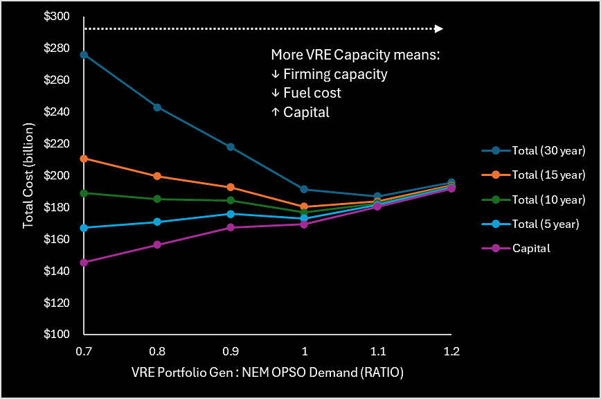
Figure 10 – VRE Portfolio Capacity: Sensitivity Analysis
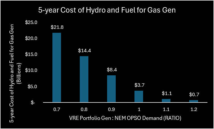
Figure 11 – 5-year Cost of Hydro and Fuel for Gas Gen (Billions)
Wind to Solar Ratio
The total output of each modelled portfolio was set to NEM OPSO demand + 10% for the wind-to-solar ratio sensitivity analysis. The system was modeled with 0%, 23.3%, 50%, 75%, and 100% solar. This was done by scaling the solar and wind portions of the Sharpe-ratio optimised portfolio accordingly. Notably, the Sharpe-Optimised portfolio (i.e., 23.3% solar) exhibited the lowest cost over any period greater than 5 years. The effects of increasing solar were:
- Slightly reduced capital. Capital reduction is tempered by the fact that solar has lower capacity factors, so the required portfolio capacity to meet demand increases with increasing solar % of portfolio.
- Increased reliance on hydro/gas/storage to supply power during significant shortfall overnight and decreased daylight hours in winter, and therefore:
- Significantly higher gas demand and long-term fuel costs.
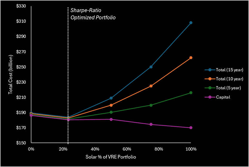
Figure 12 – Solar % of VRE Portfolio: Sensitivity Analysis
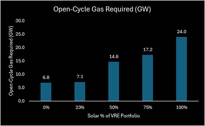
Figure 13 – Open Cycle Gas Capacity Required with Increasing Solar % of VRE Portfolio
Optimised System
Based on the sensitivity analysis, a system with VRE portfolio scaled to meet 100% NEM OPSO demand over the 2025 calendar year was selected for further analysis. Due to Hydro running out in December in this scenario, the December dispatch order was varied, leaving storage until last (same as March-August). This ensured sufficient capacity for handling longer negative runs in December, minimizing the gas power requirements in those instances.
Figure 14 summarizes the properties and performance of the optimised system over the 2025 calendar year. We have a 56 GW capacity VRE portfolio with a capital cost of $123 billion. The capital cost of firming capacity required to support this VRE portfolio is $46 billion (hydro excluded). As discussed in the sensitivity analysis, there were systems available with lower upfront cost, but once fuel costs were incorporated over 10+ years, this system was the cheapest.
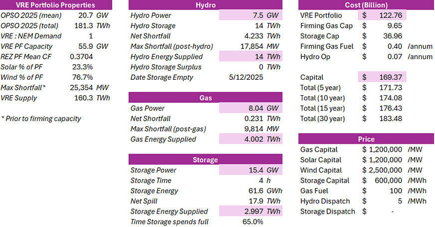
Figure 14 – Summary of Optimized System (Costs, Capacities, Energy Supplied)
Figure 15 illustrates the energy supply for a 2025 average day, with firming capacity generally kicking in for the evening peak demand period and then (mostly hydro) continuing to supply overnight while solar is at zero. All pretty stock standard. Figure 16 and Figure 17 illustrate the supply seasonality. Hydro supply is highest March through August, when hydro is first (and storage last) in the firming dispatch order. Storage is highest in the months when it is at the front of the firming dispatch order.
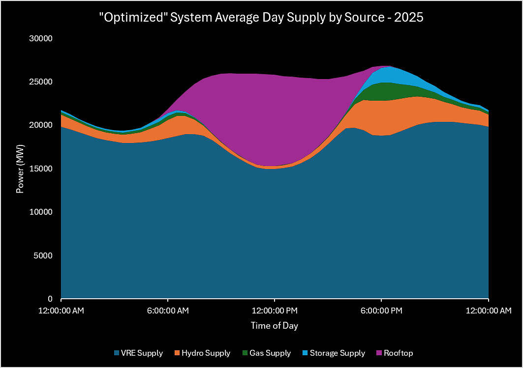
Figure 15 – “Optimised” System, Average Day Supply by Source – 2025
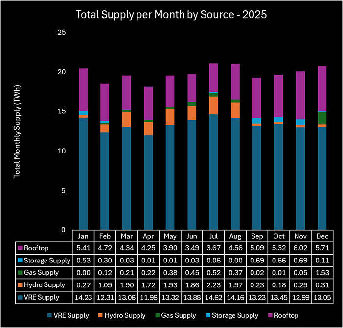
Figure 16 – “Optimised” System, Total Monthly Supply by Source – 2025
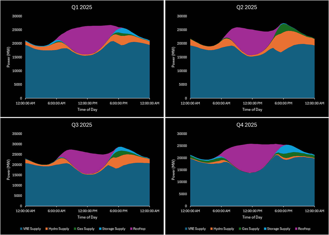
Figure 17 – “Optimised” System, Average Day Supply for Calendar Year 2025 by Quarter
Key Assumptions / Limitations
- 2022 ISP demand, solar, and wind trace data is used. Future iterations of this work will update all underlying data to reflect changes in the 2024 Draft ISP.
- Transmission costs and losses need to be incorporated in a future iteration of this work. We understand that this will prove a pivotal piece in portfolio optimisation, particularly given the (potentially unrealistic) geographical distribution of our hypothetical VRE generation network in relation to the demand centers.
- Recommend further optimisation of firming capacity dispatch order, which is currently relatively static, aside from moving storage up the order during months of increased sunlight. Once a more realistic firming capacity dispatch order algorithm is in place, storage capacity needs to be further optimised.
- Storage round-trip efficiency needs to be incorporated.
[1] 15.4 GW of storage meets 99% of shortfall, post-VRE.
About our Guest Authors
 |
David Leitch is Principal at ITK Services. He has 33 years of experience in investment banking research at major investment banks in Australia. He was consistently rated in the top 3 for utility analysis between 2006 and 2016.
David has been a client of ours, and a fan of NEMreview, since 2007. He has been a long-time contributor of analysis over on RenewEconomy, and very occasionally contributes to WattClarity! You can find David on LinkedIn here. |
 |
Paul Bandarian is a versatile analyst with 7 years’ experience in the mining industry and a proven track record in implementing data-driven strategies across multiple sectors. He is now working as an independent energy analyst with a focus on the NEM. |
That is an insanely large amount of money to produce a system that is less reliable than the fossil fuel generation system we had in place up to 2010.
And does it also take into account the shorter lives of these renewables which means we would need to be spending a significant portion of that capital outlay again every 10-15 years, in addition to having to transport and dispose of the wind and solar components?
It isn’t a particularly large amount of money, replacing the coal we had in 2010 almost all of which will have to be replaced by 2035 would cost about $100-$120bn in today’s money not including new mines or wate supplies or coal rail tracks. Combined with the operating costs at today’s coal prices would mean that the plants have a breakeven of $120-180/MWh. Firmed wind and solar can comfortably make money at $100 without suffering 2GW trips.
Peter Farley, you’ve done it again!
“Firmed wind and solar can comfortably make money at $100 without suffering 2GW trips.”
That’s right, once we have 10,000 km of new transmission lines reaching the REZs, we can enjoy $100 energy! I’m sure that transmission lines will be both dirt cheap and timely. That maths definitely adds up.
And I’m sure that this high quality transmission line will not increase our chances for transmission line failures the next time there is a freak storm.
I also like the way you implicitly blame Loy Yang for what happened on the 13th 😉
There are five big variables which are difficult to quantify which will mean that the transition is different and almost certainly quicker and cheaper than the above model suggests.
1.How much of the current “offpeak” demand which keeps coal plants going at night will be shifted to daytime “solar soaker” rates
2. What is the optimum expenditure on existing hydro eg the upgrade of Clover could be just the start of hydro upgrades.
3. Will the perception of grid unreliability drive overinvestment in behind the meter generation and storage, which will supply 20%+ of total demand and clip peak demand by 2-5 GW
4. Will detailed economic analysis drive developers toward different configurations of wind and solar farms optimized for output in suboptimal conditions rather than just adding storage to conventional designs?
5. Will the TSO’s suddenly discover dynamic rating, reconductoring and storage as transmission to speed up transmission capacity increases
@Peter Farley
1) None. With all the GIGAWATTS of capacity already in the NEM that your lobby promotes, you’re not making a dent in off-peak demand. Battery ENERGY is almost negligible when compared to coal plants.
2) Optimum expenditure? How about we use Snowy 2.0 as a proxy and go with $10 billion and a 10 year lead time.
3) Perception of grid unreliability? I guess what happened in 2022 was just a fantasy of mine. Clip peak demand by 2-5GW? You’re literally just making up numbers now.
4) LOL!!! All the best wind and solar regions are already taken. There’s nothing you can do about it, pal. That’s why your lobby wants the heavy 10,000km transmission line project subsidised.
5) “Suddenly discover”? That sounds like very sound reasoning to scrap all coal. Hopefully we’ll suddenly increase our transmission!
I will certainly be interested in seeing how this changes in future iterations with transmission requirements modelled – as you mention, the results will likely be very different.
I would note that if you are designing a system like the one your model has chosen, where there are subregions that are substantially underserved with local generation and require near-permanent access to generation that is physically remote, that leads to critical transmission infrastructure that has to be substantially overbuilt, to allow for some transmission paths to be out of service for scheduled maintenance while still remaining resilient to events that trip some of the remaining paths.
To incorporate transmission I think the offshore region(s) will need a definite location as well.
It would also be interesting to start the VRE portfolio with existing/committed VRE projects as well rather than completely ‘from scratch’. This may not change much, of course.