
With the impacts that transmission limitations have had recently on many renewable generators whether operating, in construction, or proposed, it’s not surprising that the arrival of a new constraint affecting solar and wind generators in south west NSW and north west Victoria was newsworthy – at least in the arcane context of the NEM – at the end of last week.
The constraint, going by the snappy name N^^N_NIL_3, was described by Paul McArdle in this WattClarity post, and even made news on RenewEconomy.
However this one is a little different from some of the system strength constraints that have had significant effects on renewable generators in South Australia and North Queensland, and I’ll use it as a case study for how constraints operate in general and what this one might do.
I’ll assume that readers have reasonable familiarity with the NEM dispatch process and how spot prices are set, but haven’t necessarily delved into the nitty gritty of constraints.
The purpose of constraints
As Paul explains here, constraints tell the market optimization algorithm NEMDE (short for NEM Dispatch Engine) what combinations of dispatch targets (operating levels set by NEMDE for scheduled or semi-scheduled generators and loads) it can choose in its search for least-cost dispatch. NEMDE operates with literally thousands of different constraints active in any given 5 minute Dispatch Interval (DI), and many of these reflect limitations of the transmission network, expressed as combinations of operating levels for specific generator and load combinations that are compatible with secure levels of transmission flows throughout the network.
A NEM network constraint is expressed mathematically as an inequality
Left Hand Side (LHS) <= Right Hand Side (RHS)
(in some cases instead of “<=” we might see “=” or “>=”)
The LHS expression contains entities that NEMDE can control as outcomes of the dispatch process – typically target output (measured in megawatts, MW) for generators etc. The RHS expression contains things that NEMDE can’t directly control such as transmission line limits or actual metered flow levels.
NEMDE’s objective is to minimize the overall “cost” of dispatch, where offer and bid prices of generators and loads are used to measure this cost. NEMDE must ensure that it picks not simply the lowest cost combination of bids and offers which satisfy demand, but the lowest cost combination which also satisfies (if possible) every single active constraint. If a set of dispatch targets would violate a constraint (result in LHS > RHS above), NEMDE must attempt to find a different set that satisfies that constraint while minimizing any extra cost in doing so.
The N^^N_NIL_3 constraint
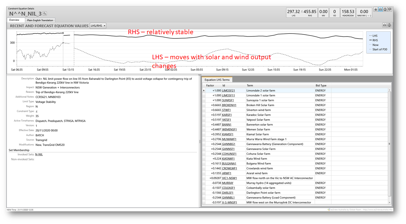
With that very quick overview, let’s look at N^^N_NIL_3. Here’s how it’s presented in Global-Roam’s ez2view market viewer software. I’ve annotated some key features of this particular view.
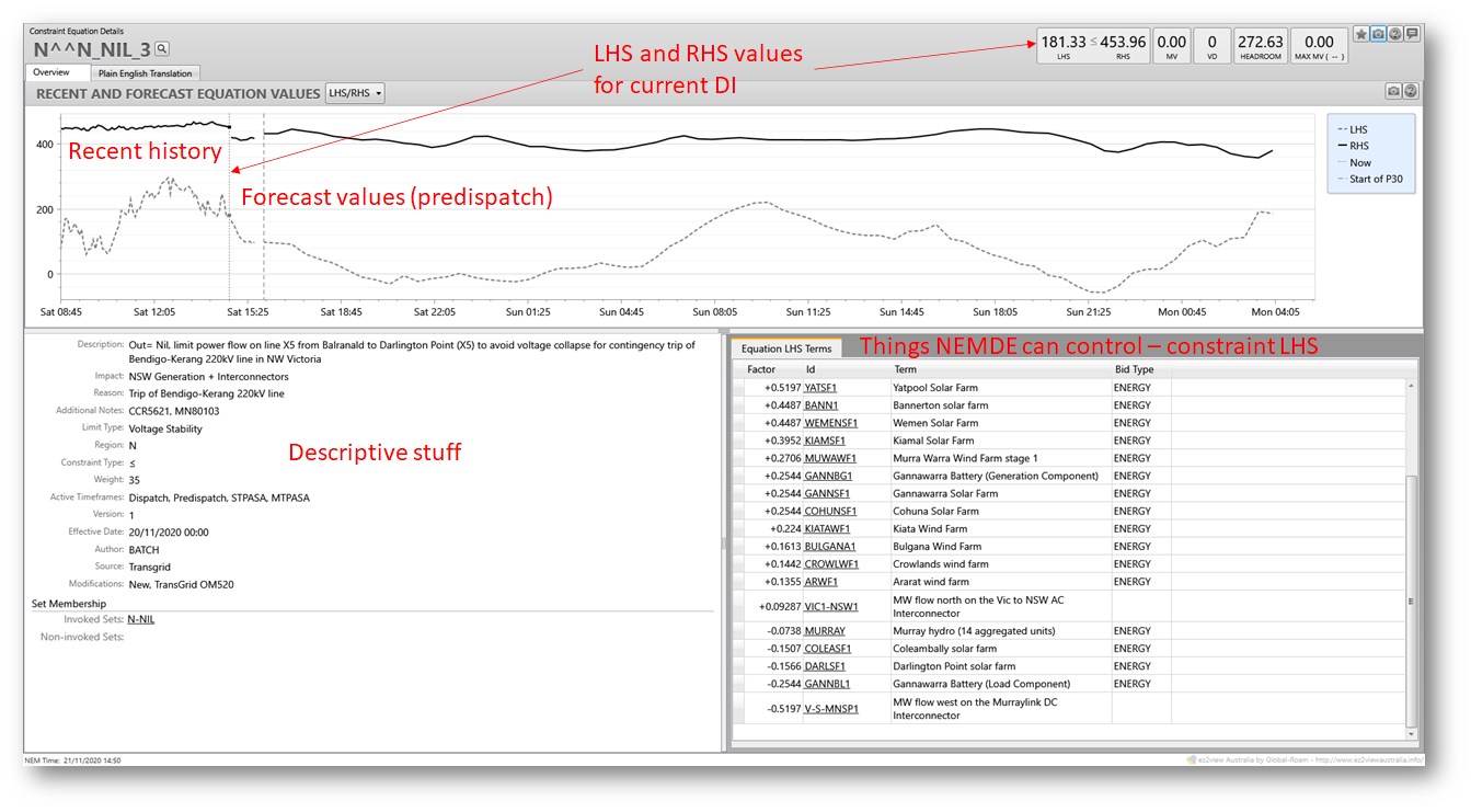
In the top part of the view we see current values for the LHS and RHS of the constraint, with a chart of their recent and predicted values. Since in this example the LHS is well below the RHS throughout, the constraint is non-binding – it hasn’t forced and isn’t forecast to force NEMDE to vary anything away from its least-cost solution (there may of course be other binding constraints in the same DI that have affected NEMDE’s dispatch solution).
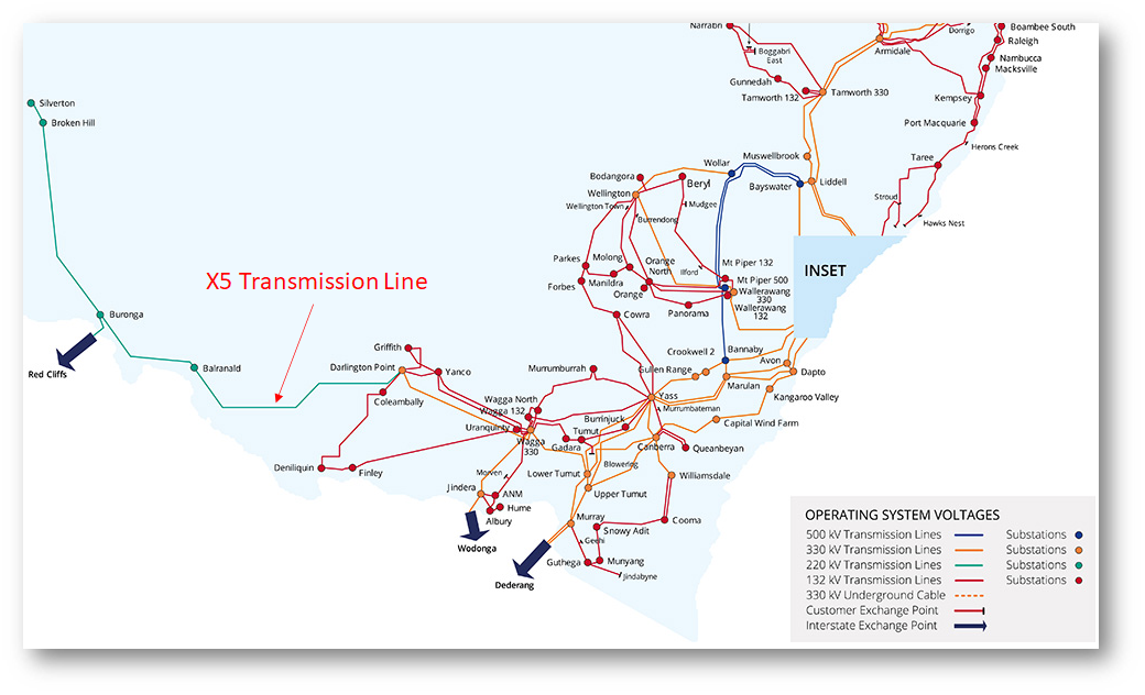
All I’ll point out from section labelled the “Descriptive stuff” is that the purpose of the constraint is to “limit power flow on line X5 from Balranald to Darlington Point”. The schematic map below of Transgrid’s NSW network shows the location of this line, which is clearly important in transferring power between south-western NSW or north-west Victoria (via Red Cliffs) and the rest of NSW.
At the bottom right of ez2view’s constraint details view in the prior chart was a panel showing “Equation LHS terms” – comprising things NEMDE can directly control in the dispatch solution, being a series of energy outputs (targets) for various generators and loads, as well as flow levels on a couple of inter-regional interconnections: VIC1-NSW1 (Victoria to NSW) and V-S-MNSP1 (the Murraylink DC interconnector from Vic to SA). Associated with each of these items is a Factor or constraint coefficient which multiplies the target value. The overall constraint LHS value is just the sum of these coefficient x target terms. The reason for this specific set of generators loads and interconnectors appearing in this constraint is that their locations mean that they directly affect power flows on the target X5 transmission line, with their coefficient values derived from power flow analysis.
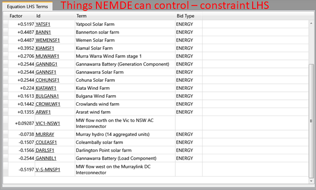
Mathematically-minded readers may notice that the constraint LHS is a linear expression, and needs to be in this form because NEMDE uses linear programming to perform its dispatch optimisation.
It should be clear that dispatch levels for generators, loads, and interconnectors in this LHS expression might be affected by this constraint if it were binding. While it’s non-binding, the constraint is not forcing any of NEMDE’s targets for these entities away from what would otherwise be least-cost dispatch.
But where does the constraint’s Right Hand Side come from? Remember that this contains things like line transmission line limits or flows that NEMDE doesn’t directly control, but has to try to “live within” while finding a least-cost solution.
If we flick ez2view’s constraint viewer to its “Plain English Translation” tab, most people’s first reaction is to laugh, because what appears isn’t really English, let alone plain:
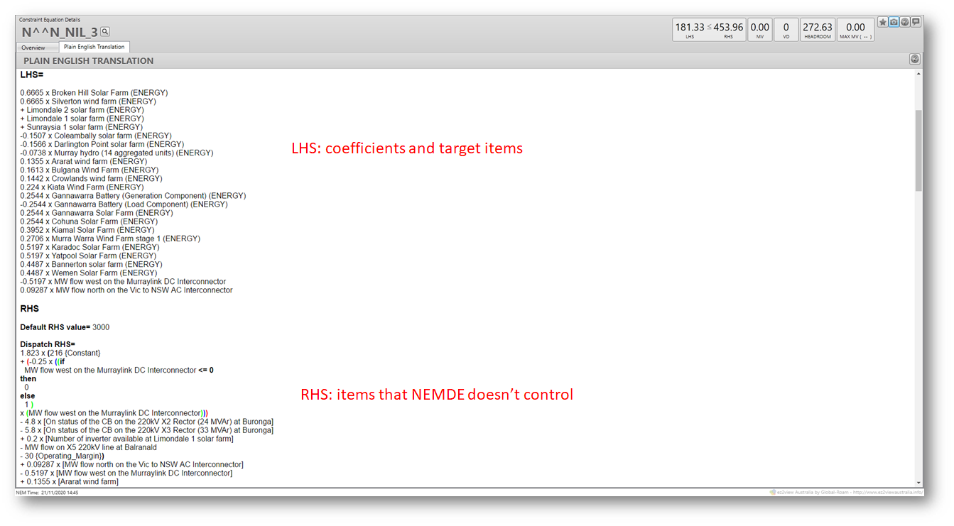
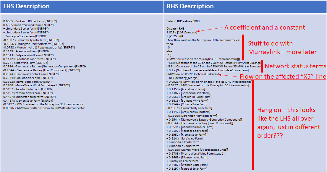
The LHS terms and coefficients appear in slightly different format, but the main new thing in this view is a description of the constraint RHS. This isn’t completely visible above so I’ve pulled out this “Plain English Translation” of the RHS into the table below, alongside the LHS. I’ve also added some annotations to the RHS, which still looks like a mess at this point.
WTF (Wait, There’s Feedback)
A key thing that stands out in this description is that the RHS seems to contain a complete copy of the LHS – just in different order. That seems crazy.
But there’s a subtle difference, because the LHS terms are the target levels for output and flows that NEMDE’s optimization sets for the various generators loads and interconnectors, to be reached at the end of the DI, whereas the RHS terms are metered actual values for the same items at the start of the DI. And whilst NEMDE directly controls the end-of-interval targets, its dispatch algorithm obviously can’t change start-of-interval actual measurements.
So those “echoes” of the LHS appearing on the RHS are measurements which NEMDE doesn’t directly control, but what are they doing there? To answer this, remember that a constraint is just a mathematical inequality:
LHS <= RHS
and rearranging this inequality, we can take those “echoed” start-of-interval metered values from the RHS across to the left (with signs changed). This turns the LHS into a sum of targeted changes over the dispatch interval for each entity, multiplied by the relevant coefficient. For example for Broken Hill Solar Farm we would get
0.6665 x [Broken Hill Solar Farm (target) – Broken Hill Solar Farm (actual)]
or written more simply
0.6665 x Δ Broken Hill Solar Farm
where Δ signifies change over the DI. NEMDE can control these changes by changing the end-of-interval target values. So the constraint is in effect telling NEMDE to limit the sum of changes in LHS items, multiplied by their coefficients, to less than a certain value (the remaining RHS terms after moving the “echoes” to the left). I’ve restated the constraint LHS and RHS this way below, and also decoded the “if – then – else” bit dealing with Murraylink:
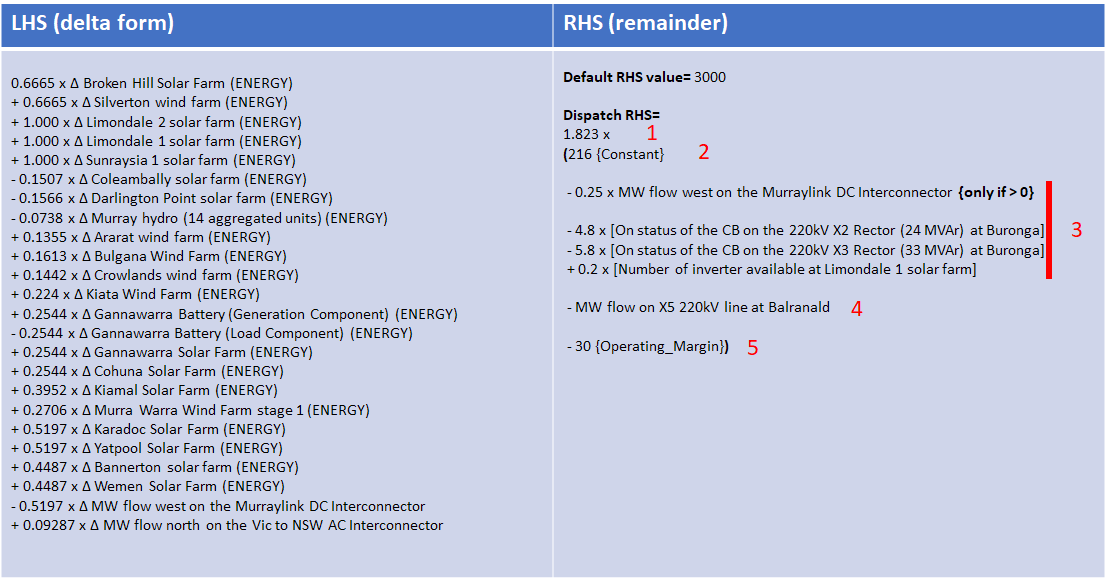
The remaining RHS has five distinct components which I’ve labelled
- A coefficient, 1.823 – this is there for conventional reasons (in order to make the LHS coefficient with largest absolute magnitude equal to either +1.000 or -1.000; but we could divide both sides of the constraint inequality by 1.823 and its overall effect wouldn’t change)
- A constant, 216, which in this case is something to do with the maximum secure flow on the X5 transmission line
- Some terms to do with network conditions which may vary that maximum secure flow (the term involving Murraylink is a little more complex but leave that aside for now)
- The measured actual flow on the X5 line (subtracted from 2 + 3 above)
- An “operating margin” constant of 30, also subtracted
When combined, items 2 through 5 represent remaining headroom available on the target X5 transmission line at the start of the DI, because they essentially amount to:
Maximum secure flow +/- adjustments for network conditions
Minus
Actual measured flow
Minus
an “operating” (or safety) margin
And this in turn explains why the constraint really deals with changes (“deltas”) in the controlled quantities, because it is essentially requiring:
Increase in X5 line flows due to output changes over the DI <= Headroom on X5 line at DI start
Although AEMO and others call this type of constraint a “feedback” constraint, because values for left hand side entities appear to be “fed back” into the RHS of the constraint equation, the purpose of this feeding back is much easier to understand when the constraint is rearranged to deal with changes in dispatch quantities.
(Technically, the constraint ends up being written the way it first appeared above because any quantities NEMDE doesn’t explicitly control in a dispatch interval – like start of interval metered actuals – have to go into constraint RHS values, which get calculated before NEMDE then runs its optimization of LHS targets.)
Who gets affected when the constraint binds?
Changes in the controlled elements on the LHS of N^^N_NIL_3 would lead to changes in flows on the X5 line – with the coefficients on the LHS terms related to how much the line flow changes for a unit output change at each generator, load etc. And with only a certain amount of headroom on the target line, the constraint is asking NEMDE not to change outputs in ways that would use up more than that headroom and violate the constraint.
As mentioned earlier, when the constraint is non-binding under NEMDE’s least-cost solution, there’s no need to modify targets for its affected entities. But the real question is what changes would NEMDE have to make when the constraint is violating, or threatening to?
To understand this, we first need to think about whether increasing or decreasing target MW values on the LHS would help ease the constraint. The constraint would violate if
LHS > RHS
so in order to reduce the LHS, NEMDE would need to reduce LHS targets with positive coefficients, or increase targets with negative coefficients. These reductions and increases are algebraic ie -20 MW < -10 MW < 1 MW < 5 MW. This is important because interconnectors can have negative or positive targets depending on the direction of flow. By convention, target MW values for generators and loads are always positive or zero.
It should also be clear that a 1 MW target change in items whose coefficients have largest absolute magnitude will make the biggest difference to the LHS. In N^^N_NIL_3 these would be the Limondale and Sunraysia solar farms with coefficients of +1.000. So would these always be the farms whose output NEMDE would seek to wind back if it needs to reduce the LHS by some amount?
It all depends on cost
Not necessarily; we also need to consider cost, because NEMDE will seek to alter targets in a way which minimises the incremental cost to the dispatch solution. Let’s suppose that the three solar farms with coefficients of +1.000 have all offered their energy at $5/MWh while the Broken Hill Solar Farm, coefficient +0.6665, has offered energy at $40/MWh. We’ll also need to know the spot price in NSW so let’s suppose that is $50/MWh.
Now, a 1 MW reduction in dispatch target (away from what would otherwise be least cost) at Limondale or Sunraysia farms would reduce the LHS value by 1 MW (coefficient +1). NEMDE’s cost function views this as a “saving” (because it’s taking less energy from this source) of
$5/MWh (offer price) * 1 MW ie $5 per hour.
To have the same effect on the LHS (reducing its value by 1) NEMDE could instead reduce the output target at Broken Hill Solar with its lower constraint coefficient by 1 MW / 0.6665 = 1.5 MW. This would reduce NEMDE’s cost function by
$40/MWh (offer price) * 1.5 MW per hour or $60 per hour.
But NEMDE also has to keep supply and demand balanced, so if it reduces targets at one of the solar farms in NSW, it has to increase NSW supply somewhere else by the same amount. Now the $50/MWh NSW spot price comes into play, because the spot price is the marginal cost of supplying extra energy in NSW by definition. If NEMDE winds back Limondale or Sunraysia by 1 MW, the spot price tells us that hourly cost of making up the output from elsewhere must be
$50/MWh * 1 MW = $50 per hour
whereas winding back Broken Hill Solar by 1.5 MW (to achieve the same 1 MW change in constraint LHS) will require another 1.5 MW of supply from elsewhere, costing
$50/MWh * 1.5 MW per hour = $75 per hour
Netting these changes in offer costs and “make-up” energy, we see that the net additional cost of reducing the constraint LHS by 1 MW by changing output at Limondale or Sunraysia, versus changing output at Broken Hill given their relative offer prices and constraint coefficients is
-$5 (offer saving) + $50 (make-up energy) = $45 per hour for Limondale or Sunraysia
-$60 (offer saving) + $75 (make-up energy) = $15 per hour for Broken Hill
so in this case NEMDE would not wind back output at Limondale or Sunraysia, despite their larger coefficient, but instead prefer to wind back Broken Hill Solar’s more expensive output because this yields a smaller increase in NEMDE’s cost of dispatch.
Incentives to rebid
If you’ve got this far, you should be able to see from this example that NEMDE’s choice of which LHS entity or entities to vary, in order to satisfy a constraint that would otherwise violate, depends on (at least) their coefficients, their offer prices, and the relevant regional spot price(s). So it’s certainly not a simple matter of “which farm has the largest constraint coefficient”.
But you can probably also work out that if the constraint is violating or binding, generators with positive coefficients that do not want their output wound back might choose to offer their energy more cheaply, by rebidding at low or negative prices, because this will give NEMDE less incentive to reduce their output – in fact it sees reducing output at a negative offer price as a cost not a saving.
Following this logic, all generators with positive coefficients under a binding constraint may end up rebidding to the market floor price of negative $1,000/MWh to give NEMDE the maximum disincentive to wind their output down. In this case NEMDE will revert to choosing the generator(s) with the largest positive coefficient(s), since these require the smallest change in MW output to impact the constraint LHS by a given amount and hence the smallest cost to dispatch.
But what about interconnectors?
Interconnectors often appear in a constraint LHS, as they do in N^^N_NIL_3, but have two important differences from generators and loads – their target MW values can be negative or positive, and they don’t have associated offer prices for NEMDE to use in its cost calculation. So how does NEMDE deal with them in a binding constraint?
The answer is that the change in dispatch costs associated with modifying interconnector targets simply involves the spot price difference between the two interconnected regions.
Considering the VIC to NSW (VIC1-NSW1) interconnector, the convention on flow direction is that positive values or targets mean flow from the first (Victorian) to second (NSW) region and vice versa. So algebraically reducing the flow target on this interconnector means either lowering positive flows (Vic to NSW) or increasing the magnitude of negative flows (NSW to Vic) while maintaining overall supply / demand balance in each region. In either case this requires reducing supply from other Victorian sources (eg generation) and increasing other supply in NSW. NEMDE sees the cost of these changes as just
[change in target MW (-ve for reduction)] * ([Vic spot price $/MWh] – [NSW spot price $/MWh])
(Ignoring any changes in inter-regional losses for simplicity)
Although generators and loads potentially affected by a constraint can choose to rebid, altering their offers in ways that might strongly discourage NEMDE from varying their target MW, interconnectors in the same constraint don’t have offer prices. So depending on constraint coefficients and relative spot prices, they might be first cab off the rank for changes when the constraint binds or violates.
Consider Vic to NSW flows under the N^^N_NIL_3 constraint which has a coefficient of +0.09287 for this interconnector. Assume that NEMDE is looking for a net 1 MW reduction on the constraint LHS and that the Vic spot price is $30/MWh while in NSW it is $40/MWh.
To get a net reduction of 1 MW on the LHS, the change in target flow across VIC1-NSW1 would have to be -1 MW / 0.09287 = -10.77 MW, with less Victorian supply required from other sources (the negative change means exports to NSW are decreasing, or imports into Vic are increasing) and more supply required in NSW. The net change in hourly dispatch costs is given by these changes in other supply and regional spot prices:
-10.77 MW x $30/MWh (saving in Vic where less generation is required) + 10.77 MW x $40/MWh (extra cost in NSW where more generation is required)
= $107.70
If generators under the constraint are all offering at low enough prices – say -$1,000 /MWh – then changing interconnector flows may well be the cheapest option for resolving the constraint and therefore what NEMDE chooses to do – even though this change in flow would be “counter-price” – requiring “make-up” supply in the more expensive NSW region and a supply reduction in the cheaper Vic region. If a large enough reduction is needed on the constraint LHS, NEMDE could end up swinging the Vic-NSW interconnector flow quite strongly in the counter-price NSW to Victoria direction, with the size of this swing related to the inverse of the interconnector’s constraint coefficient. Which looks rather like the tail wagging the dog – but that’s the outcome of following the dispatch logic.
So how likely is this N^^N_NIL_3 constraint to actually bind?
We saw above that there seemed to be plenty of headroom on the N^^N_NIL_3 constraint over the short historic and forecast window charted. But what about the future – how likely is this constraint to bind and force some of the impacts discussed above?
Without getting into highly detailed market modelling we can get a rough idea by looking at example values for the constraint LHS and RHS, and how these might change under different conditions. Here’s a snapshot of the constraint for the 12:35 DI on 21 November, when its LHS was at a relatively high value but still well under the constraint RHS
I’ve noted on the chart that the constraint RHS value doesn’t fluctuate all that much whereas the LHS clearly moves up and down, with ups broadly corresponding to daylight hours – this is what we’d expect for the LHS given its preponderance of solar farms with relatively large coefficients. (If you’re wondering why the RHS doesn’t fluctuate similarly even though it contains “feedback” metered output values for the same solar and wind farms, that’s because the RHS also includes the negative of flows on the X5 line, and the whole point of the combination of entities and coefficients in this constraint is that changes in their output should be reflected in changing flows on that line)
Under what conditions might the LHS – 297 MW in the example DI – get high enough to cause the constraint to violate? Self-evidently, if we saw more solar and wind output at farms with larger positive coefficients. And importantly, some of the large solar farms under this constraint are not yet fully operational – Limondale 1 (220 MW), Sunraysia (200 MW) and Kiamal (200 MW). What might happen when these are fully up and running?
To illustrate, here’s a table showing the LHS contributions from the affected entities for the example 12:35 DI shown, highlighting solar and windfarms that were not operating anywhere near maximum capacity, together with a calculation of how those LHS contributions would change if all the solar and wind farms in the constraint were operating at 60% of their maximum capacity:
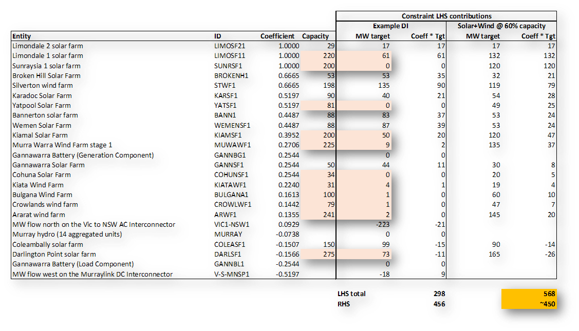
The calculation shows that this 60% capacity across the board (setting aside what might be happening with interconnectors or Murray power station) would be enough to lift the LHS up to or above the RHS value (which is just notional in the 60% solar + wind case, but probably in the right range), potentially causing the constraint to violate and forcing NEMDE to start altering targets for some entities, using the logic described above.
So we could expect to see this constraint starting to regularly impact dispatch on sunny and windy days, especially once the large solar farms mentioned above are fully commissioned. Perhaps I’ll come back to this post in a month or two and see if this bold prediction is correct.
In Summary
Constraints are one of the more complex features of NEM dispatch, and can tend to seem impenetrable. While their “Left Hand Side” terms and coefficients might appear clear enough, Right Hand Side expressions can be mystifying, and understanding the overall effect of any given constraint or working out which elements on the LHS might be most affected appears to require guesswork, or simple – but sometimes misleading – rules of thumb like “largest effect on generator with highest coefficient”.
But if you’ve persevered to the end of this case study, first of all congratulations, and secondly I hope you have a little more insight into what drives constraint formulation and operation in general, and what we might see happen specifically when and if N^^N_NIL_3 binds.
About our Guest Author
 |
Allan O’Neil has worked in Australia’s wholesale energy markets since their creation in the mid-1990’s, in trading, risk management, forecasting and analytical roles with major NEM electricity and gas retail and generation companies.
He is now an independent energy markets consultant, working with clients on projects across a spectrum of wholesale, retail, electricity and gas issues. You can view Allan’s LinkedIn profile here. Allan will be sporadically reviewing market events here on WattClarity Allan has also begun providing an on-site educational service covering how spot prices are set in the NEM, and other important aspects of the physical electricity market – further details here. |
just gone up another level, started thinking this may be megawattclarity, but stuff it, terrawattclarity Allan! clarity indeed.
Thanks Victor! Bit more of a mouthful.
So Paul, Allan – (maybe even Ben B or Alex W at AEMO) – any thoughts on whether we will get into a round of debate about the merits or otherwise of having an interconnector term with such a small co-efficient, but wide range (much bigger than any generator) on the LHS? It’s above the threshold, but at 0.09287 you don’t get the best relief – and we have already seen similar equations swing the interconnector 1800MW in a TI recently. economics vs physics anyone? Should interconenctors have a different threshold given their range? do these swings cause any other power system issues, now, will they in the future?
Thanks to Allan for a very clear and concise description of despatch constraints. In a well-ordered system the proposed interconnector to SA would hopefully alleviate this constraint.
Time will tell.
P.S. I propose we refer to the area west of Wagga as the ‘Triangle of Tribulation’.
I’d wondered about ‘polygon of pain’, Malcolm.
I never understood why this ever needed to be a “polygon of pain”. From what I can see there is no reason why AEMO could not have operated the Balranald-Buronga line normally-open at Buronga (with a backup auto-close scheme). This would force the power flow away from X5 up through the high-capacity Dederang interconnector instead, potentially avoiding any curtailment. Maybe I am missing something?
I’ve just dialled back in after 14 months of retirement and it’s great to know that the neurones haven’t completely turned to mush in that time. Thanks Allan for a great explanation. I’m thinking of using it to dazzle some mates when someone asks why their bills are so high or how the NEM works. I am very happy to now be just a spectator though I do miss the access I used to have to NEM data.