Examples of self-forecasting behaviours – part 5 – afternoon underestimations

Background

This is the fifth in a series of articles (all collated in the category ‘Games that Self-Forecasters can Play’) to help illustrate some of the different self-forecasting approaches that we’re aware of, approaches that were discussed back in 2022 and, in many cases, are still observed in 2025.

In each example we have used real data – but have taken steps to anonymise the data (obscured the DUID and date, and normalized the capacity of the unit) because the purpose of these articles is not to point the finger at any particular unit. The purpose is help readers understand approaches that have been in use.

Readers should keep firmly in mind that:

• As noted before, it’s impossible to know motive – but does not stop us guessing.
• Also, on Sunday 8^th June 2025 we see the commencement of Frequency Performance Payments – which:
  • Does both:
    • Changes the approach to apportioning Regulation FCAS costs; and
    • Establishes a payments and cost recovery mechanism for Primary Frequency Response.
  • And in doing so, it also retires the use of the ‘Frequency Indicator’ for apportioning regulation FCAS costs which (in our view) has been exploited for for the behaviours we part of the games note above.
  • As a result of this change, we may see changes in these approaches.

Today’s example: afternoon underestimations

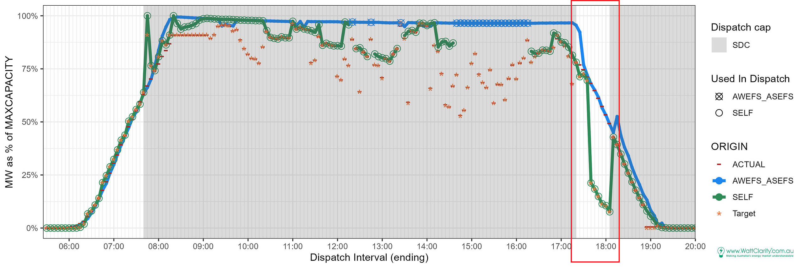
On this day, the solar farm had been under tight control with semi-dispatch cap conditions lasting most of the day and targets were visibly constrained.

Intervals 17:40 to 18:05 stand out because the forecast appeared to be biased low – self-forecasts suddenly dropped roughly 30-40 percentage points and then increased a short time later.

All the while actual output remained predictably in line with the pattern of the setting sun (and the AWEFS_ASEFS forecasts).

Impacts on share of Regulation FCAS costs

In his earlier article ‘Games that self-forecasters can play (Part 1 – An Overview)’, Paul identified two legs that form the foundations for self-forecast biasing:

1. Minimising a (Semi-Scheduled) DUID’s share of Regulation FCAS costs
2. Avoiding AEMO suppression
   with both legs needing to be played in tandem.

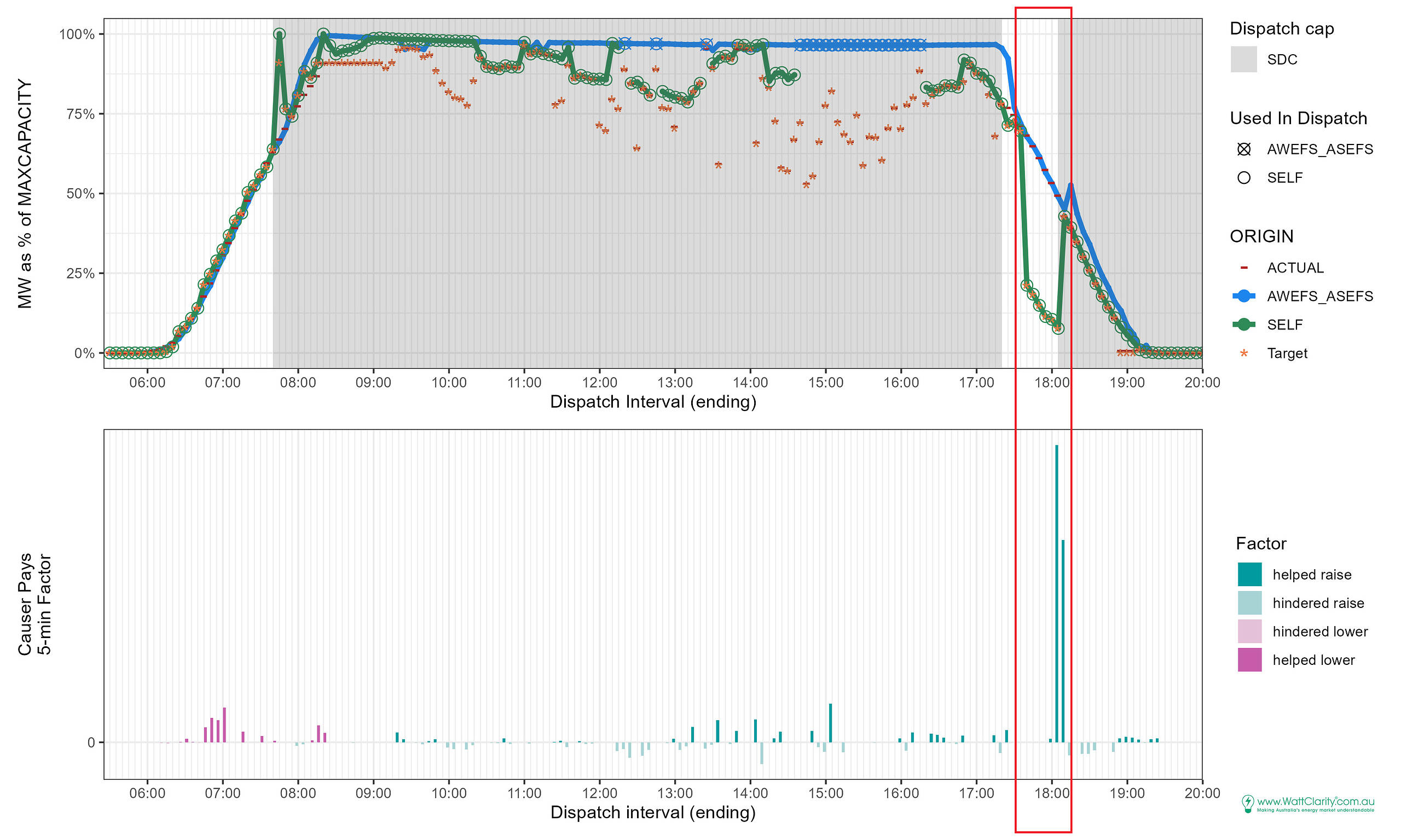
With this biasing event driving forecast error we look to impacts on the 5-minute causer-pays factors for a motivating outcome.

We inspect the causer-pays factors because this event happened when Causer-Pays was the mechanism for allocating costs of Regulation FCAS (prior to June 8 2025).

From June 8, 2025, the mechanism is Frequency Performance Payments.  

The 5-minute Causer Pays factors earned over this time are presented below.  We find two intervals lucked out (‘helped raise’ in interval 18:05 and 18:10). Other intervals in the ‘biased-low’ event appear to have missed out on earning positive factors. We explored some reasons for this happening in Examples of self-forecasting behaviours – under the hood of part 1.

Impacts on forecast accuracy recovered earlier

The impact on forecast performance, of the late-afternoon biasing is evident in the lower panel of the chart below.   The green bars are greater than 40% in magnitude meaning self forecast performance has taken a considerable hit in those intervals when biasing appeared implemented.

One possible way to regain performance against/relative to the AWEFS_ASEFS forecast appears in the chart below, purple boxed-period. The strategy has three components:

1. Bias availability low,
2. Receive a low target,
3. Match output to target, thereby making the higher AWEFS_ASEFS forecast look bad.

With the lens I’m looking through, this pattern appears most clearly over the 10:00 to 13:30 intervals.

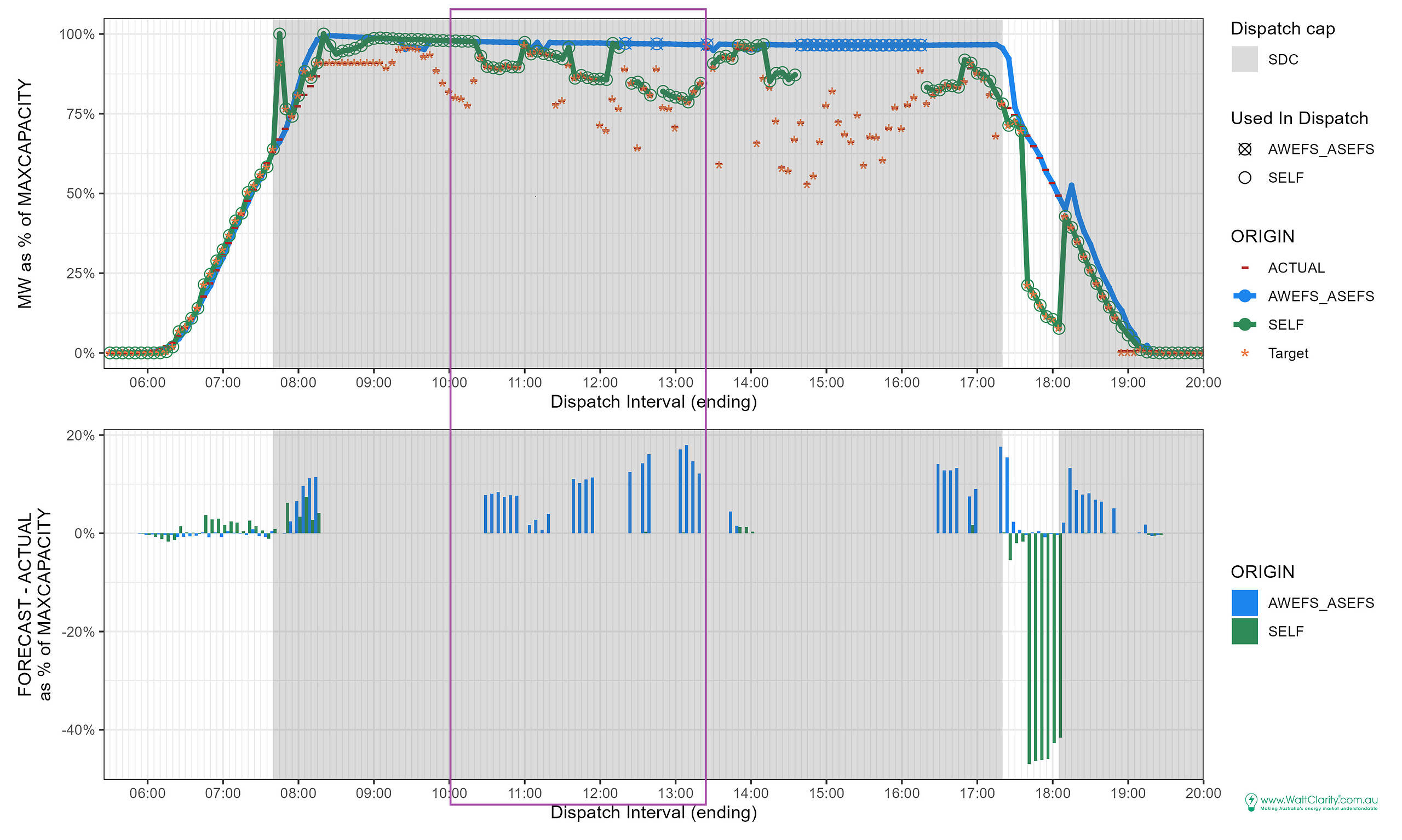
Under what the AWEFS_ASEFS forecast appears to think are clear skies (because of the flat top, indicating maximum availability for that time of year), the self-forecast dips low for brief periods. The example range is 10:00 to 13:30.

With output matching a lowered target, the “forecast – actual” difference is, in contrast, large for the AWEFS_ASEFS forecast.

Note that forecast differences are not eligible for performance comparison when the unit’s target is less than the unit’s availability. We’ve applied this in the chart above. This condition eliminates intervals when the unit is constrained, output is not expected to match unconstrained availability. The intervals around 09:00, and also 14:00 to 16:00, are examples of this.