Examples of self-forecasting behaviours – part 2 – relative accuracy

Background

This is the second in a series of articles (all collated in the category ‘Games that Self-Forecasters can Play’) to help illustrate some of the different approaches that we’re aware of.

In each example we have used real data – but have taken steps to anonymise the data (obscured the DUID and date, and normalized the capacity of the unit) because the purpose of these articles is not to point the finger at any particular unit. The purpose is help readers understand approaches that have been in use.

Readers should keep firmly in mind that:

• As noted before, it’s impossible to know motive – but does not stop us guessing.
• Also, on Sunday 8^th June 2025 we see the commencement of Frequency Performance Payments – which:
  • Does both:
    • Changes the approach to apportioning Regulation FCAS costs; and
    • Establishes a payments and cost recovery mechanism for Primary Frequency Response.
  • And in doing so, it also retires the use of the ‘Frequency Indicator’ for apportioning regulation FCAS costs which (in our view) has been exploited for for the behaviours we part of the games note above.
  • As a result of this change, we may see changes in these approaches.

Today’s example: Relative accuracy

Part 2 in this series presents an example of self-forecasting that supports improved relative forecast accuracy.

This is relevant because a sufficient level of forecast accuracy is needed to pass the ongoing weekly performance assessments.

In Part 1 we saw how forecast accuracy can be sacrificed for other means.  At some point, that accuracy needs to be recovered. Otherwise AEMO-suppression is risked through failing a performance assessment.

In the chart below, we observe the self-forecast sitting persistently below the AWEFS_ASEFS forecast and much closer to the self-forecasts.

This is highlighted with the yellow boxes.

This leads to the self-forecasts being frequently closer to actual output, boosting performance relative to the AWEFS_ASEFS forecasts.  Particularly periods 12:55 to 15:15 and 16:25 to 19:20.

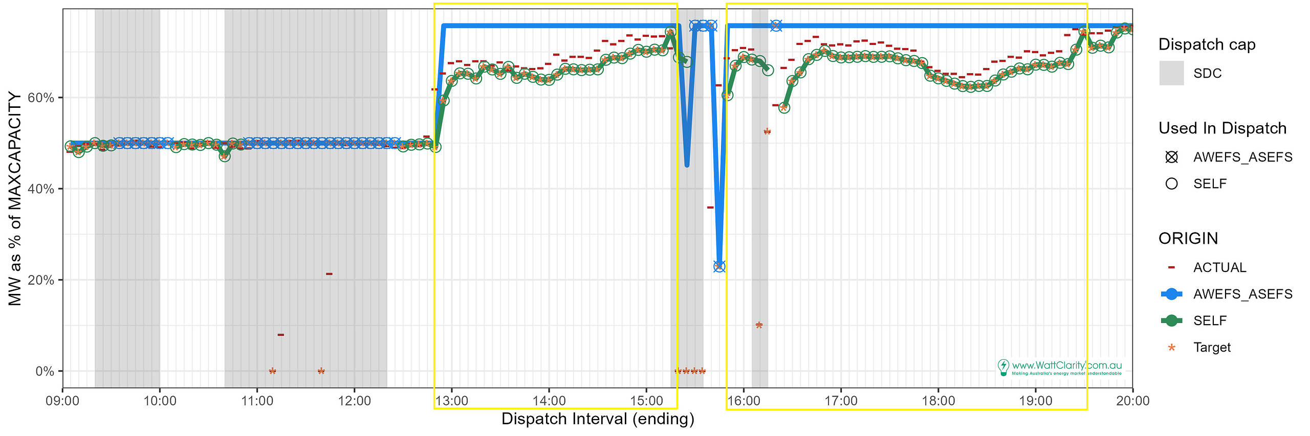
I’m arguing self-forecast biasing (biasing low) was applied here yet the magnitude is difficult to quantify. More than one contributing factor may have played a role after 12:50:

1. The AWEFS_ASEFS forecast appeared (relatively) off. A local limit was in place at 75% of max capacity from 12:55 onwards and it appears the AWEFS_ASEFS forecast believed there was enough wind to deliver output at least at that level. It may have been missing information, preventing it from producing a lower forecast.
   1. Meaning, the self-forecast may have been more realistic, or
2. The self-forecast was biased low, achieving possibly two aims;
   1. A lower dispatch target, so that actuals could be higher than target, supporting frequency raise and,
   2. To afford better performance against actual output, relative to the AWEFS_ASEFS forecast.

Differences show a bias

Differences are calculated as forecast – actual, charted below.

Furthermore, differences are only calculated when the target is not below the forecast used in dispatch. In other words, when the unit’s target is not constrained. Hence some gaps are present in the chart.

In the case of 2.b., the chart indicates the self-forecast’s differences were smaller than those of the AWEFS_ASEFS forecast.

The differences would contribute to improved lower RMSE and MAE scores, relative to AWEFS_ASEFS, in the weekly performance assessment.

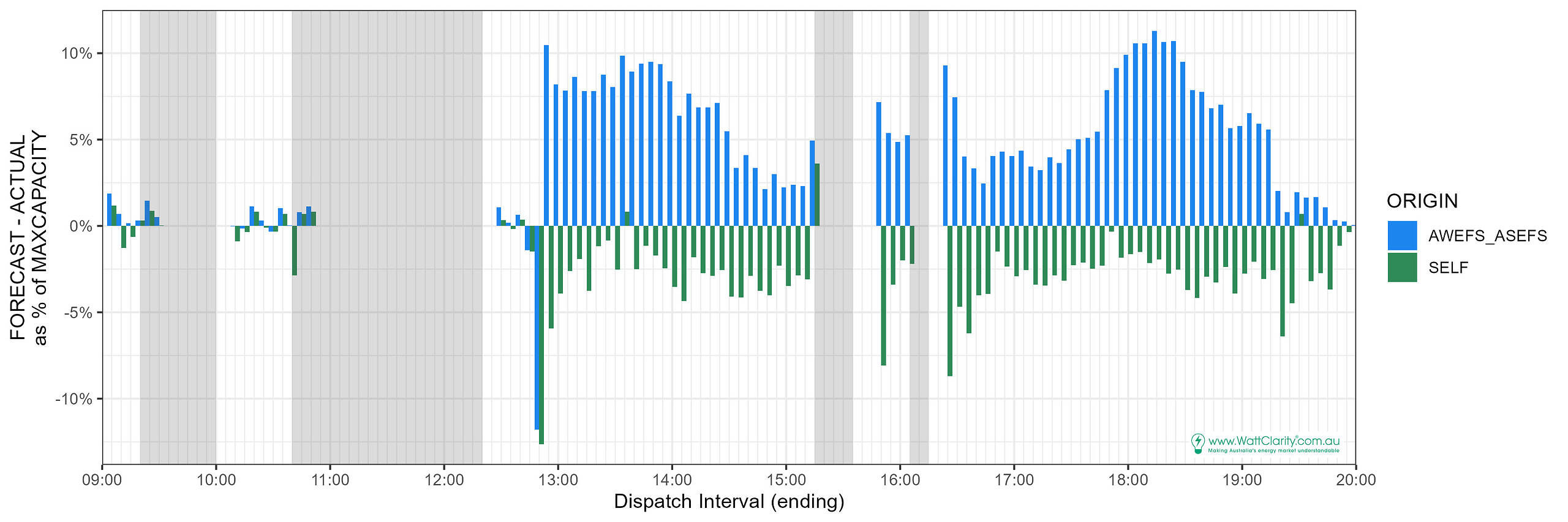
While differences occurred in both forecasts, the self-forecast’s differences were consistently negative (forecasts were below actual output levels). The persistent bias in differences suggests a bias in the self-forecast.

Supporting frequency raise too

While not the focus of this article, the self-forecast levels supported positive deviations from targets, which in turn supported positive impacts on Causer-Pays 5-minute factors.

We observe this in the chart below. The intervals with ‘helped raise’ align with the biased-low periods.

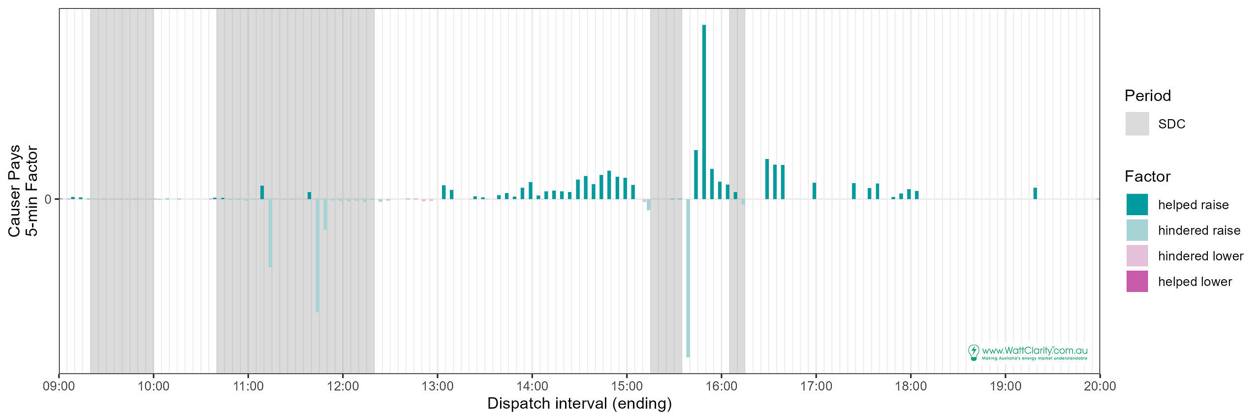
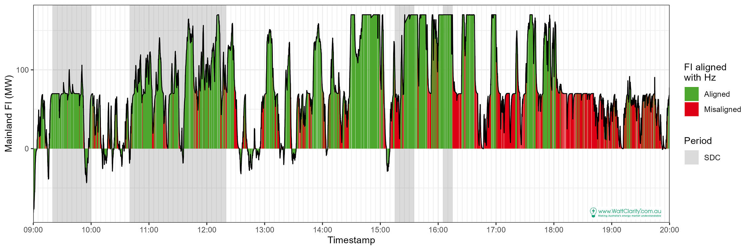
A strong tendency for positive Frequency Indicator (FI) values played key large role in that persistent ‘helped raise’ outcome.

Note that ‘helped raise’ is derived from 4-second measurements when a positive deviation aligns with the frequency indicator (FI) and the FI is aligned with actual system frequency need.   If system frequency is not aligned, the 4-second measurement is not used.

Furthermore, too many misaligned measurements mean a 5-minute factor isn’t calculated.