With the benefit of hindsight – or who’d be an auto-bidder?

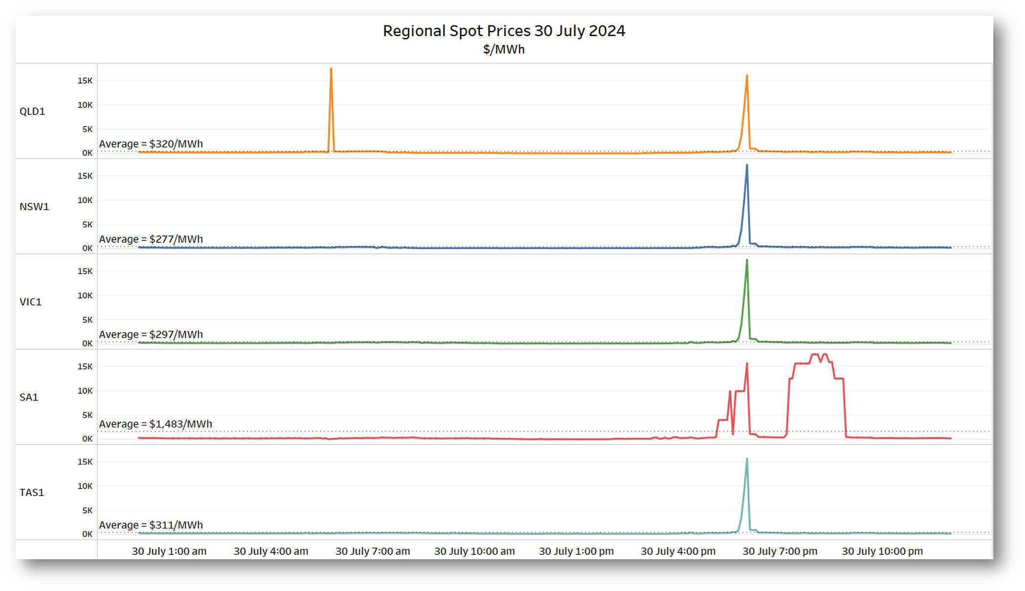
South Australia experienced two blocks of volatile spot prices on Tuesday 30 July, exceeding $1,000/MWh in 32 dispatch intervals between 17:10 and 20:50 (NEM time, or AEST). Other regions also saw a handful of high price intervals, including the notable NEM-wide event in the interval ending 18:00. The average South Australian spot price for the day was over $1,480/MWh, nearly five times higher than averages in other NEM regions.

This post picks up on Linton’s analysis of bidding in South Australia to focus on:

• The role of interconnector limitations
• The behaviour of the region’s growing battery fleet
• Some challenges arising under extreme market conditions for the ‘autobidder’ software used to manage batteries’ market dispatch

Ez2view’s NEM-wide map at 18:00 has been reproduced in a few places already, but here it is again with the interconnectors between South Australia and Victoria highlighted:

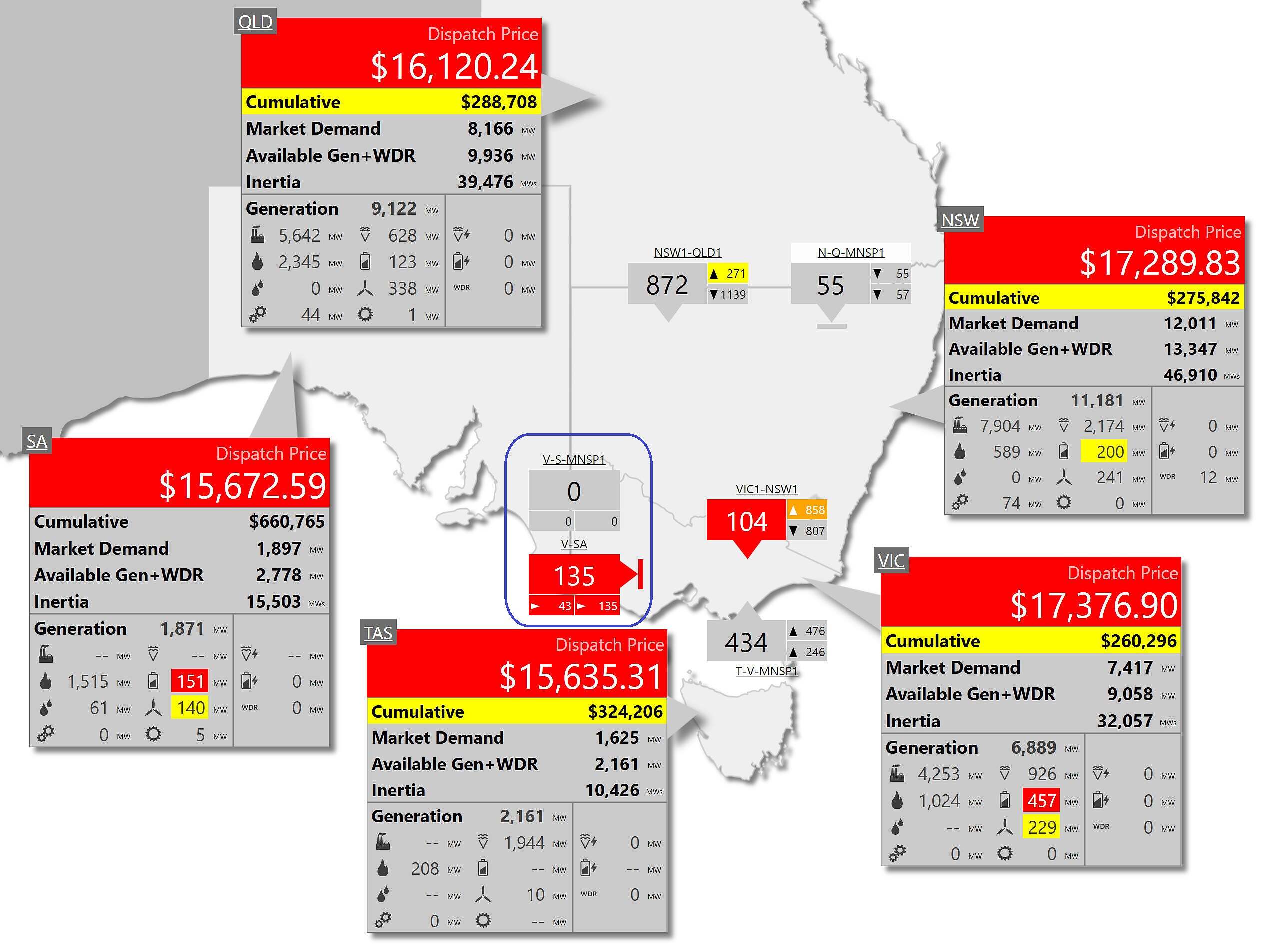
The Murraylink DC interconnector was out of service at the time, and the Heywood AC interconnection was also significantly limited by a scheduled line outage. This limitation particularly affected maximum flows from Victoria into South Australia, generally to less than 50 MW and at times forced flows from generators and batteries in south-eastern South Australia into Victoria.

These outages and limitations meant that for most of its price volatility episode, South Australia was economically islanded from the rest of the NEM. Had the Heywood interconnector been able to carry its normal ~600 MW capacity into South Australia, that region’s excess volatility would have disappeared.

As things turned out, spot prices reflected specific bidding behaviour by South Australian generators as identified in Linton’s post, particularly:

• A proportion of the thermal fleet’s available capacity being offered at five-digit price levels
• Variable contributions from the regional battery fleet

I’ll concentrate on the latter in the next section of this post.

Battery behaviour

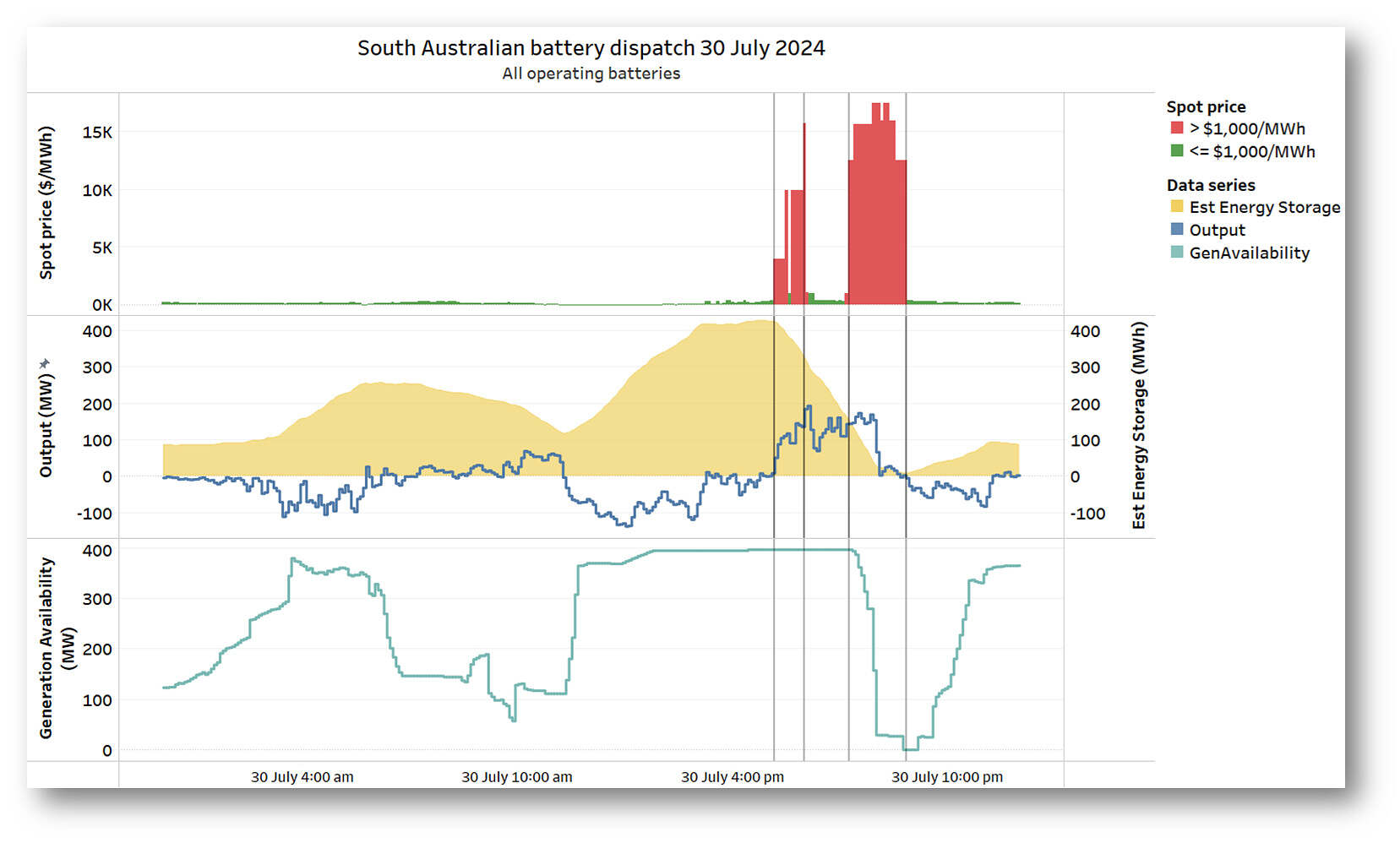
Here’s Linton’s chart of aggregate bidding and dispatch outcomes for the South Australian battery fleet:

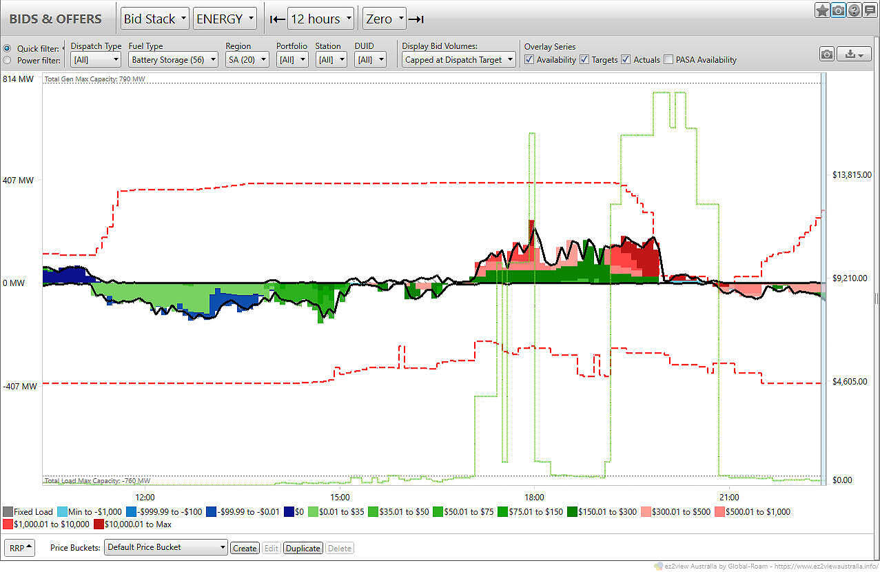
There was a maximum of about 400 MW of battery capacity offered to the market for the initial high price period, with output peaking at around half that capacity (implying that the remaining available capacity was offered at higher prices, close to the market cap).

During the second high price block starting at 19:15, batteries again initially dispatched a little under half of their maximum capacity, but fleet availability then rapidly declined, falling close to zero about halfway through this volatility episode.

This seems to indicate that, partially depleted by their initial response to the high prices from 17:10, and having continued to discharge during the period of more moderate prices from 18:05 to 19:10, the fleet simply ran out of stored energy during the second block of more extreme prices. We’ll come back a bit later to the (apparently) obvious question of why the fleet continued to discharge during the hour of ‘moderate’ prices between the two extreme price blocks, leaving themselves with insufficient stored energy to more fully capitalise on the second run of volatility.

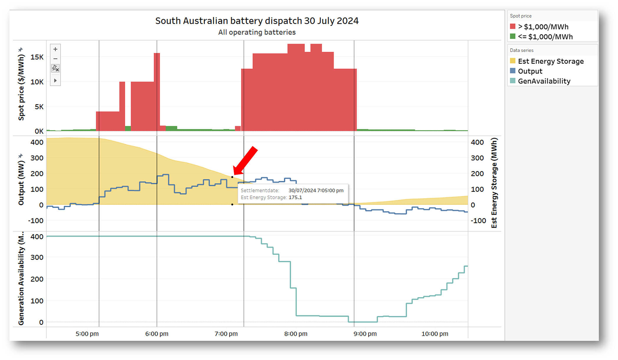
First, we can easily confirm that lack of stored energy was the issue in the case of AGL’s Torrens Island Battery, at 250 MW the largest storage unit in the region. It is now registered as a ‘Bidirectional’ unit and one of AEMO’s reported data items for these units is state of charge or stored energy level. This is graphed in the middle panel of the following chart along with its output (negative when recharging), accompanied by South Australian spot prices in the upper panel, and the battery’s offered generation availability in the lower panel:

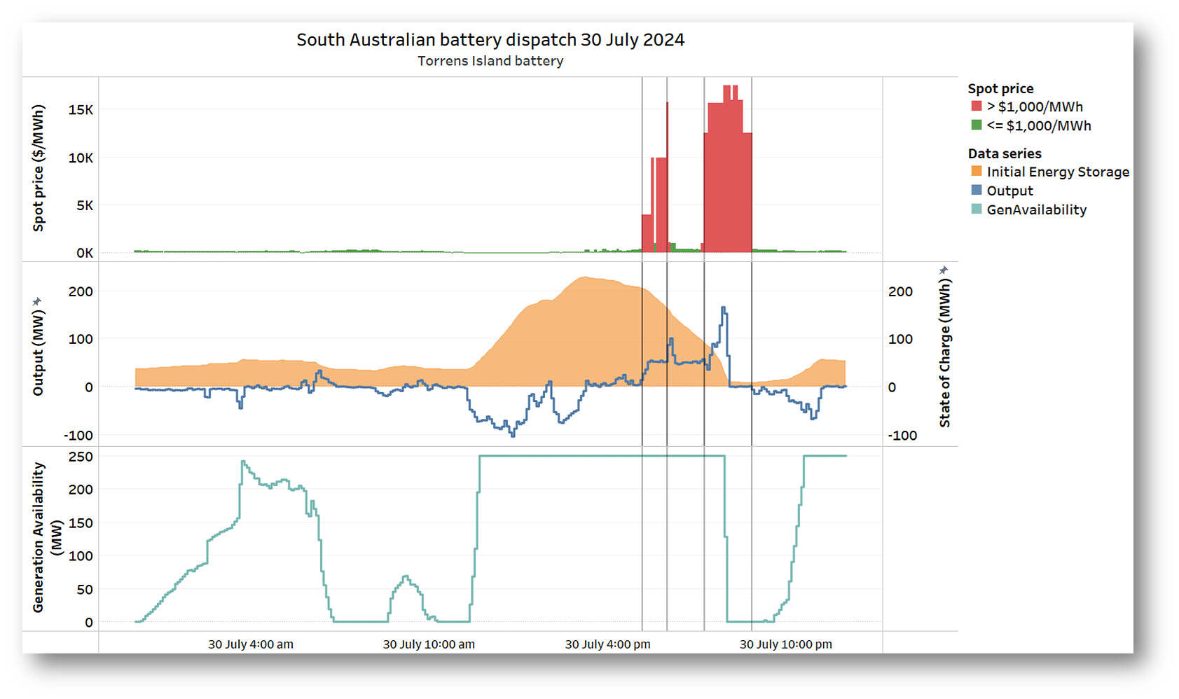
Energy stored in this battery reached 227 MWh by mid afternoon, slightly less than one hour of charge at the battery’s maximum output, and then fell through the evening volatility periods, becoming close to depleted (10 MWh) by 20:05, at which point its availability to generate not surprisingly fell to zero.

While most other batteries in South Australia don’t yet report their stored energy, with a bit of back-calculation based on output levels and calibration against the observed result for Torrens Island, we can infer the storage position for the rest of the region’s fleet to produce an aggregate view:

Since the Torrens Island battery represents about 60% of operating fleet capacity, this not surprisingly shows a very similar overall outcome – stored energy ran down over about three hours, consistent with a fleet aggregate storage duration of about one hour at maximum discharge rates, and output averaging one third of that maximum rate over the depletion period.

The next chart shows output and stored energy for individual batteries (aggregated in the case of SA Water’s fleet of small storage units):

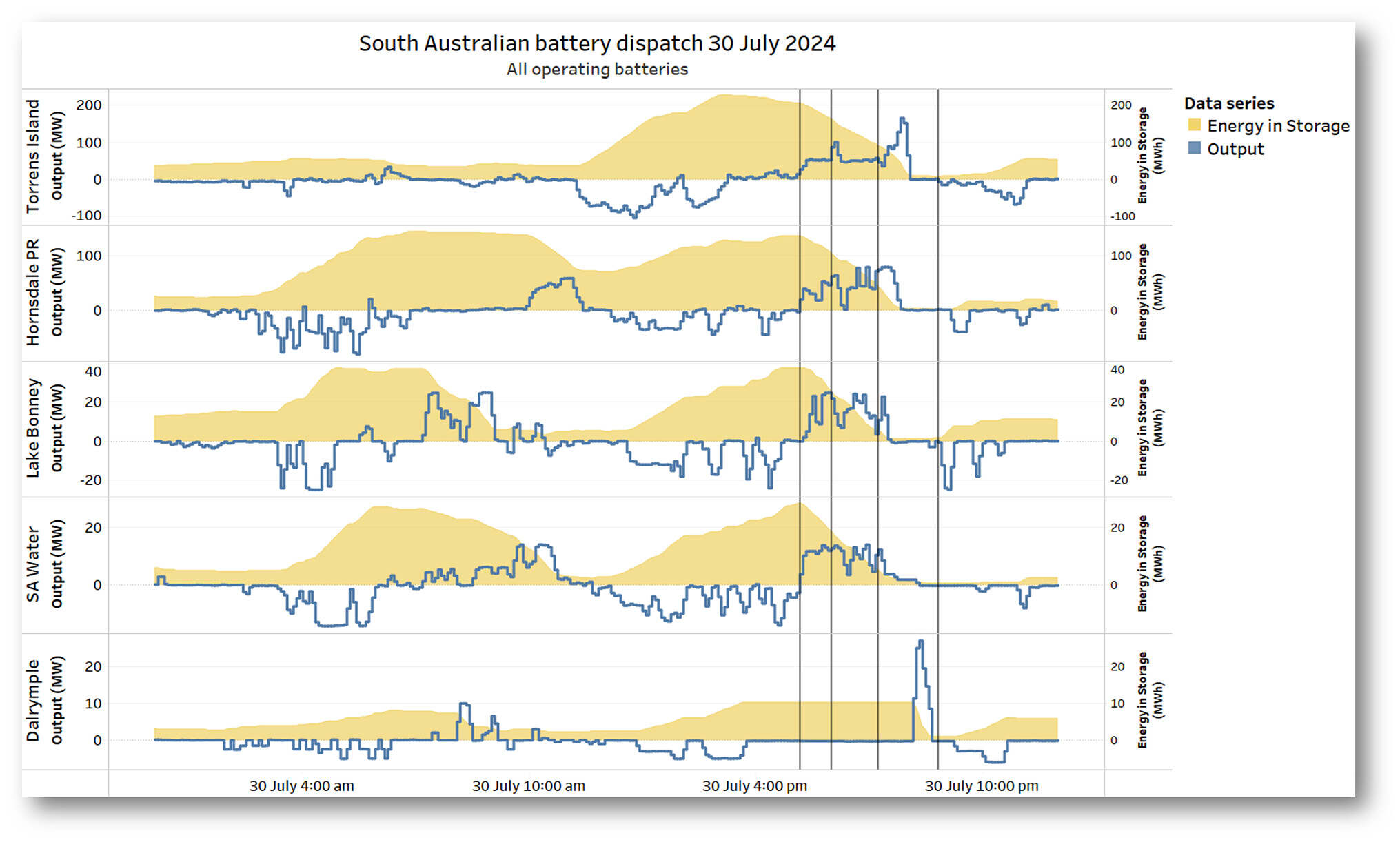
Patterns of operation are similar across the fleet, although the Dalrymple battery which has a very small storage capacity (just 20 minutes or so) only discharged at the tail end of the second high price period.

A challenge for autobidders

Overall, this episode is a neat (or perhaps messy?) illustration of the challenges for battery operators in managing a very limited quantity of stored energy* over a relatively long period of price volatility.

* Some time ago, the authors of GenInsights21 shared their Observation 5/22 about ‘the rise of Just in Time’ with readers here on WattClarity.

All the batteries in the fleet reached the start of the first volatility period holding close to their maximum charge, but then appeared to ‘waste’ nearly half of that valuable stored energy by continuing to discharge after the end of that period but before the second more extreme block of volatility arrived. Why?

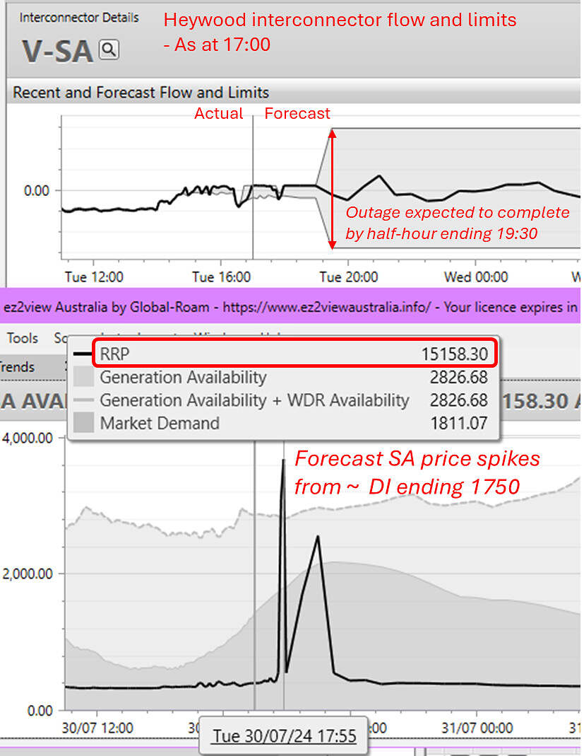
One part of the answer lies in the interconnector limitations we noted in the first part of this post. In the screenshot at the right I’ve mashed together a couple of ez2view charts showing actual and forecast flows on the Heywood interconnector, together with projected South Australian spot prices, as at 17:00 on 30 July. The forecast sections of these charts are drawn from AEMO’s predispatch (market forecast) datasets. These AEMO forecasts combine projections at 5-minute granularity for the first forward hour (updated every five minutes), followed by half-hourly projections for later times (only updated at the start of each half hour). They show the projected arrival of high spot prices within the next hour, and also illustrate that the tight Heywood interconnector (‘V-SA’) limits were at this time expected to be released for the half hour ending 19:30 (presumably by the start of that interval, at 19:00), on completion of the relevant line outage works.  This timing coincides with the retreat of projected prices from 5-digit levels.

Batteries’ autobidding software would almost certainly use these projections, probably supplemented by internal forecasts or otherwise algorithmically processed, as one input to their optimisation calculations, which are broadly aimed at achieving maximum value for battery capacity and stored energy across the NEM’s energy and FCAS markets. In the energy market, this very roughly entails a daily arbitrage cycle of recharging at times of lower spot prices and seeking to discharge when spot prices peak – in reality the optimisation involved is much more nuanced, but the basic idea of ‘buy low, sell high’ is enough for our purposes here.

Given the above view of projected spot prices, and the expected release of the Heywood interconnector limitations from 19:00 onwards, we might expect batteries’ bidding strategy over the next two hours being set up to discharge much of their stored energy at times of maximum price, before the interconnector restrictions lift. With only one hour’s worth of energy available (on average), this still requires some smart rationing of available capability, and explains why the batteries output at only up to half their maximum power during the first period of volatility. Even more so because there is no certainty about how long a period of high prices might actually last nor how high prices will actually go.

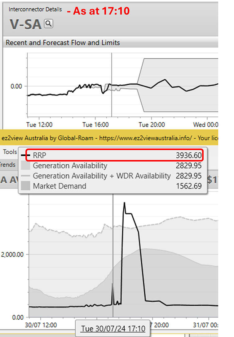
To illustrate the last point, moving forward 10 minutes shows that high prices have arrived earlier than projected, with the SA spot price at $3,936.60/MWh for the interval ending 17:10:                   At this stage the immediate forecast doesn’t show the high spot prices returning until about 17:55, but …

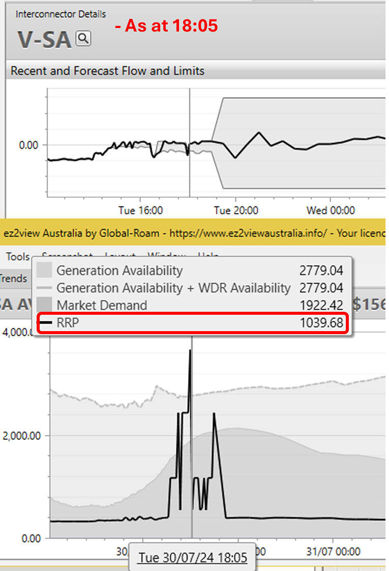
… jumping forward to 18:05, we see that prices remained elevated for almost all the intervals after 17:10:               The spot price has now fallen back to $1,039.68/MWh and projected prices over the next hour look more moderate than in the earlier projections but still in 4-digit territory. Recall from the earlier charts that at this point the battery fleet has used about a quarter of its stored energy discharging into the high prices over the previous 55 minutes.

So far the batteries’ aggregate bidding and dispatch behaviour seems sound – stored energy has been directed into the initial block of high prices and plenty held in reserve for high prices projected to occur up until 19:00 when the interconnector restrictions ease.

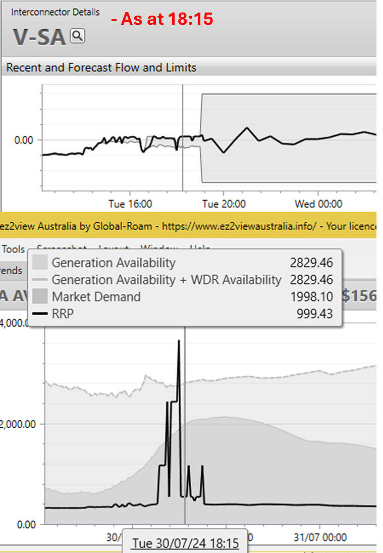
But 10 minutes later those price projections have softened considerably:                 By now the batteries’ autobidding algorithms may have collectively determined that the next 45 minutes are as long as even moderately elevated spot prices (currently $999.43/MWh) might persist, and continued to discharge energy during these intervals.

At 18:40 this strategy still looks OK – prices have retreated to $360.75/MWh and now no further price spikes are being projected:           So although batteries have run down their stored energy to about half capacity by continuing to discharge after the initial volatility period, this would appear to have realised better value for that energy than reserving it for higher prices that didn’t eventuate – so far.

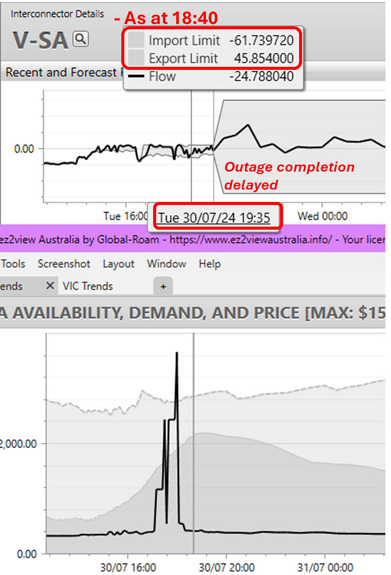But a closer look at the Heywood interconnector projection in the top panel of that last chart shows an important change – the flow limits now persist out to the end of the 5-minute predispatch projections at 19:35. These limits were originally projected to ease in the half-hour ending at 19:30, ie by 19:00. That is no longer the case, and it seems the line outage is running longer than scheduled. This means that the risk of higher prices in South Australia persists for significantly longer than previously expected, even if the current projection still shows only ~$300/MWh prices through this period.

Nearly half an hour later, prices have followed that forecast, but there is still no release of the interconnector restrictions within the next hour: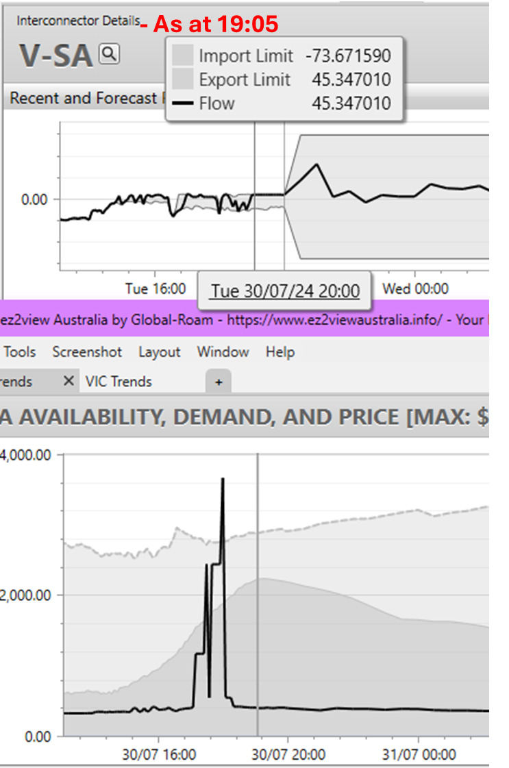

And having continued to discharge, the battery fleet is now down to about 40% of its storage capacity:

Five minutes later things go a bit pear-shaped (if you’re a battery autobidder) – price volatility suddenly reappears in the predispatch forecasts, coinciding with the continuation of the interconnector limitations until (at least) 20:00: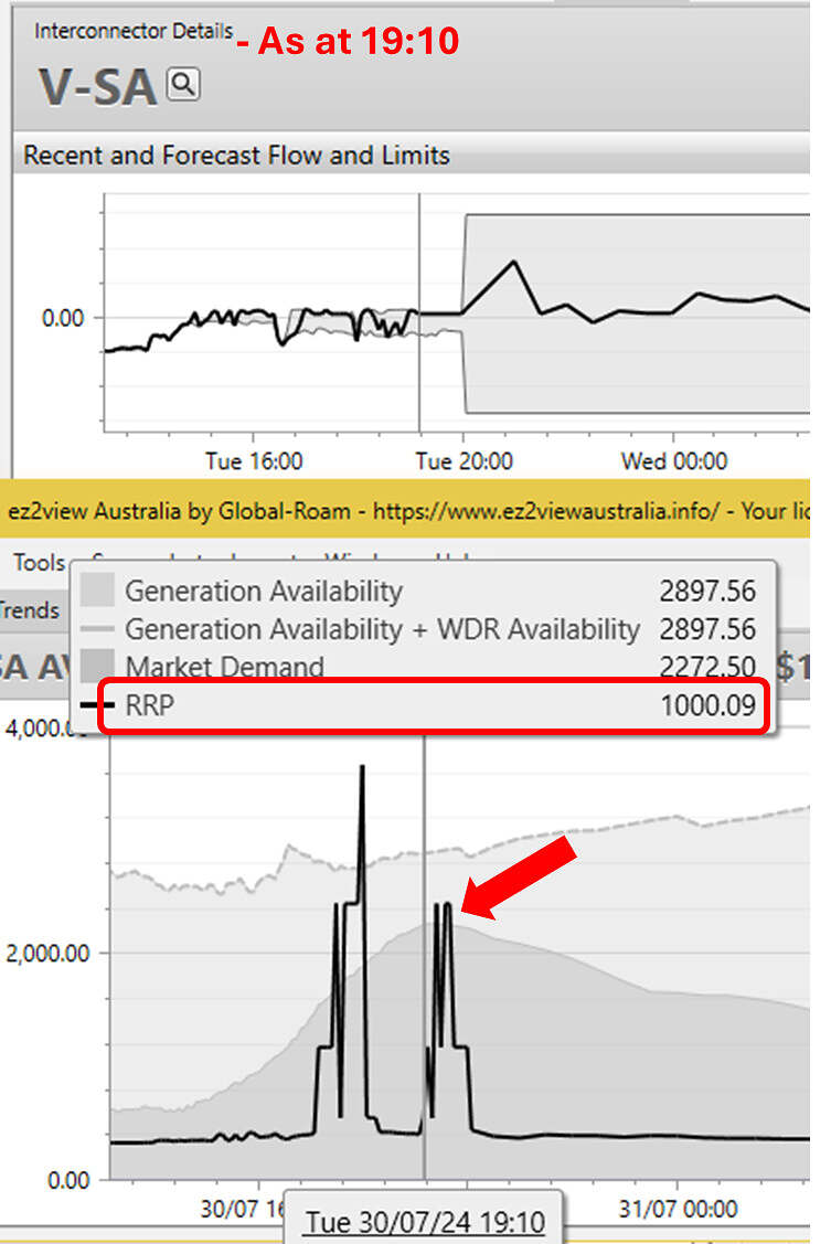

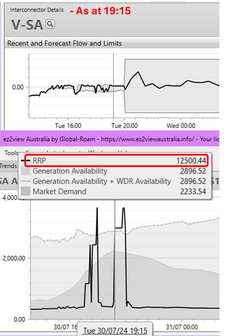
Forward another five minutes and it’s now worse than pear-shaped. The spot price is $12,500/MWh and the projected volatility block is solid at or above this price for the remainder of the outage period:               For anyone cross-referencing Linton’s article, this interval corresponds with the rebid of all the available 140 MW of gas-fired capacity at AGL’s Barker Inlet plant to the market price cap of $17,500/MWh. Probably not a coincidence.

 

There’s no point in stepping through further interval-by-interval detail from here. Ultimately the interconnector outage and limits remained in place even longer, not ending until 21:20 (dispatch interval ending 21:25), more than two hours later than originally expected. The second block of price volatility ultimately lasted 95 minutes from 19:15 until 20:50, when demand eased sufficiently for spot prices to retreat: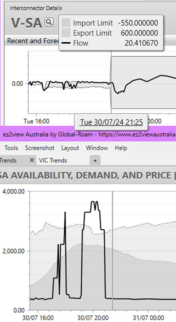

 

Conclusions – ouch

Perhaps lulled into a false sense of security by predispatch price projections that didn’t anticipate an extension of the interconnector outage (and couldn’t anticipate any generator rebidding* to leverage the impact of that extension), by the time the second volatility block arrived, battery autobidders found themselves with their storage capacity only a little over one-third full. Not surprisingly, they mostly discharged the remaining energy they had over the next 45 minutes or so, before retiring hors de combat.

For future dispatch intervals, AEMO’s predispatch projections use whatever bids are in place for those future intervals at the time the forecast is run. Participants can subsequently modify those bids at any time before dispatch (subject to a ~20-30 second technical “gate closure” window – described here as Gate Closure #2), provided they comply with the market rules concerning “good faith bidding” and the Australian Energy Regulator’s guidelines.

In summary, the episode highlights two distinct difficulties for autobidders (or even human bidders) in managing a battery fleet with relatively short storage duration:

• Even with perfect foresight, energy in storage has to be rationed across a volatility period of any significant length, limiting batteries’ ability to either profit from or suppress that volatility.
• Short storage duration significantly reduces margins for error and amplifies the risks arising from using inherently imperfect forecasts to set up and execute a bidding and dispatch strategy.

To illustrate the financial impact of these challenges, an admittedly gratuitous calculation of the revenue opportunity missed by South Australia’s batteries in discharging between the two extreme price period runs as follows:

• Between dispatch intervals 18:05 and 19:10, the South Australian fleet discharged just under 160 MWh of stored energy – about 40% of their storage capacity – which earned spot revenue of about $82,000, achieving an average price of about $520/MWh.
• Had this energy been available for discharge in the second volatility period from 19:15, it could have earned revenue of up to $2.4 million at an average price of over $15,000/MWh.

Who’d be an autobidder indeed?

=================================================================================================

About our Guest Author