Seasonality and deep storage in a highly decarbonized NEM

Summary

The main message is that wind and solar, Variable Renewable Energy (VRE) is highly seasonal in its production with much lower NEM wide production in June and July and much higher production in November and December.

So as VRE share of production increases, so too does the need for storage. The total energy supplied by dispatchable power will decline (assuming in the first instance demand is relatively flat) because existing dispatchable power loses share of the energy market to VRE, but the absolute number of dispatchable megawatts will stay relatively constant.

At very high penetration, VRE supply = VRE demand (over a year)  storage is unlikely to be enough on its own, because in some months and some consecutive months demand will exceed supply most of the time and in other consecutive months supply will exceed demand.

The result is that storage assets will end up having high (~30%) unavailability factors because they are either empty or full.

 

 

VRE is also going to change spot market pricing and flatload quarterly futures pricing

As VRE penetration increases spot prices are going to be increasingly soft in the lead up to Christmas and will tend to be higher in June and July. Initially, the June and July peak may be concealed by an excess supply of thermal generation competing for market share, but as the coal generators close the annual price peak may move from the March Quarter to the middle of the year.

We note that one competitive advantage of hydrogen, other than its low carbon status, is its low cost of storage. This makes it well suited to a seasonal role although other technologies may also come to the fore.

Finally, our modelling suggests only a limited State diversification portfolio effect.
(1)  Most obviously it’s Winter in every State in the same months, Winter may be less obvious in Queensland than in Tasmania but it’s still Winter. The NEM wide winter supply deficit can’t be fixed by building more transmission.
(2)  Equally every State will likely see over supply in late spring, early Summer. Supply portfolio optimization can help but will nowhere near eliminate seasonality.

 

Background

This note recaps a presentation from the Smart Energy conference. For that presentation we were asked to talk about problems facing utility-scale VRE developers.

Those problems transmission, and missing revenue as more supply is forced into fixed demand, are very obvious today. They were also very obvious and predictable years ago.
1)  We here at ITK wrote several notes back in 2017 and 2018 about how transmission was going to be an issue and we could have written those notes years before that, if ITK had existed then.
2)  I also interviewed Warren Lasher from ERCOT about how ERCOT, the TX, operator was able to get its competitive renewable energy zones [CREZ] established, with the appropriate transmission infrastructure, how it was done in a consensus fashion and how broadly the State of Tx has benefitted from it.

That interview is available as an episode of EnergyInsiders podcasts (>6.3 K downloads).

Interestingly I reported in one of those notes back in 2018, that the one thing the Tx guys said they wished they had done earlier was more system stability analysis. My point is there is a lot to be learned by reading up on the good and bad experiences that others have gone through and that many big problems are foreseeable and can be minimized with appropriate forethought.

In that spirit, we thought we’d talk about an issue that is small right now but without attention may become bigger. And that’s seasonality.

 

Developing the cumulative deficit graph

Our basic concept is the Cumulative Deficit. Let’s leave the national debt jokes to one side and start with NEM wide annual demand expressed here as the 7 day moving average annualized total in TWh.

 

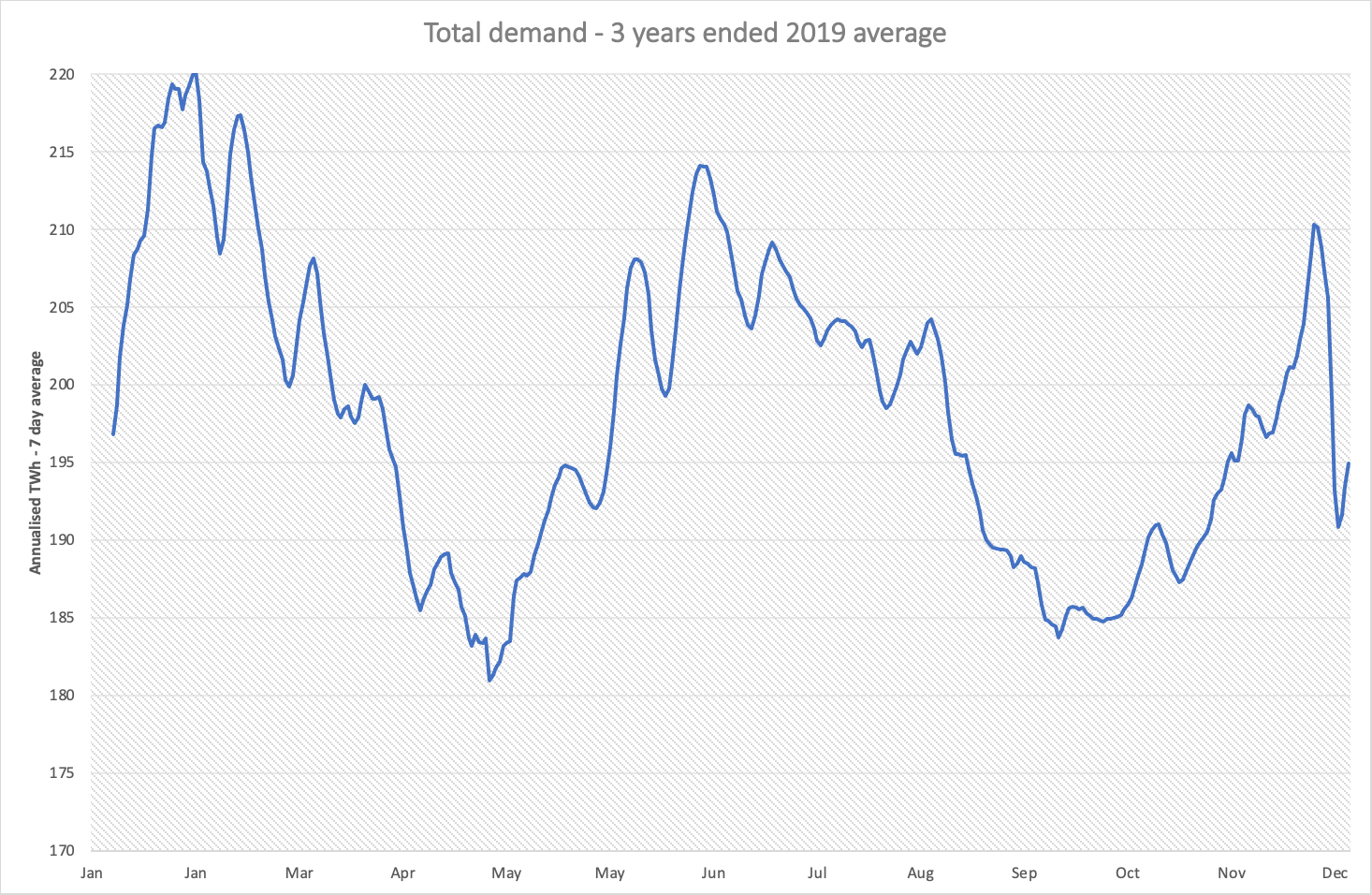
Figure 1 Source: NEMreview

 

We used three years of data ended calendar 2019. You can see the Feb peak and also the secondary winter heating peak in June and July

Next let’s look at VRE  [wind + solar] supply using the latest 12 months data to 30 August 2020. The only wrinkle is we’ve taken the Dec quarter 2019 and put it on the right of the chart and called it the Dec 2020 quarter.

 

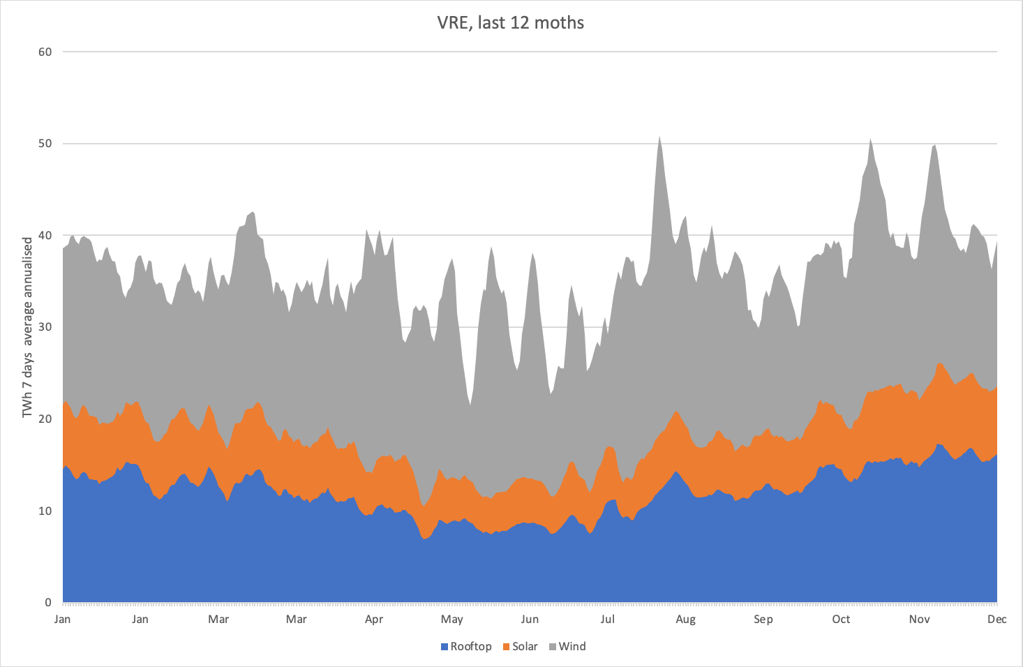
Figure 2 Source: NEMreview

 

Next we take the total of wind and solar and express it as a line graph, and use a “false zero”  vertical axis.  The seasonality of production starts to appear but still not very obvious.

 

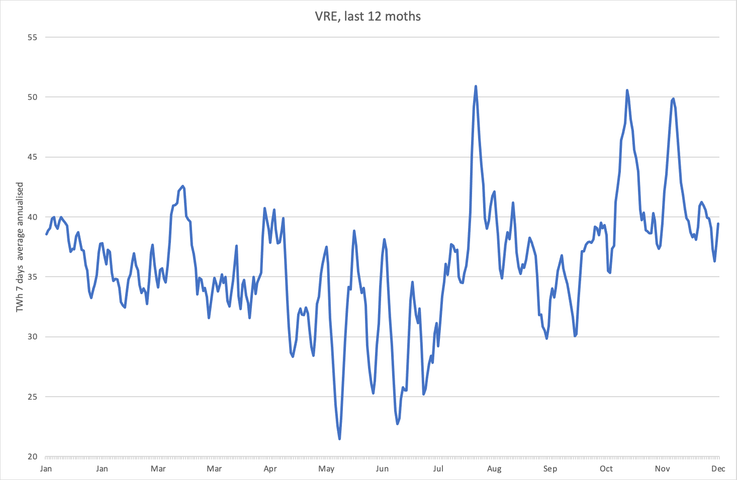
Figure 3 Source: NEMreview

 

Next, we can express  both demand and VRE supply as an index.  To do this we take the  365 day average of demand and of supply and express each average as 100. Then we measure every day’s demand relative to that year-long average and every day’s supply relative to the yearlong supply average.

By doing this both demand and supply are rebased to 100 and we can show them on the same graph.

 

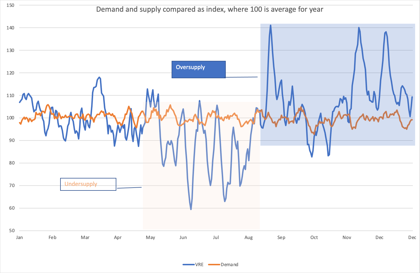
Figure 4 Source: NEMreview

 

And now the seasonality and higher volatility of supply becomes more obvious and we can’t even see the demand variability because it’s so small relative to supply.

 

Grossing up supply to equal demand with half hourly data

To move to the next stage we use the same data period  but now half-hourly data instead of day-long averages. We can compare the NEM wide, year-long, average half-hourly demand of  22 GW and total energy  over the year 220 TWh with average VRE  supply of 4.5 GW and total VRE energy of 40 TWh.  We then divide average VRE  supply 4.5 into average demand 22 to get a ratio of 5.5. So then it’s a matter of multiplying supply for every half hour of the year by 5.5 and total supply will equal total demand. Average supply will equal average demand.

 

Grossing up to 100% VRE
		NEM	VRE	VRE Grossed up
Average annual demand	GW	22.6	4.1	22.7
Total energy	TWh	199	36	200
Standard deviation	GW	3.3	2.6	14.5
Std dev % of mean		15%	63%	64%

Figure 5 Source: NEM Review

 

Although the average and total demand now equals average and total supply over a whole year there are differences every half hour either positive (demand > supply) or negative.

We can see the result for Jan 1 and Jan 2 in what’s as very standard looking chart.

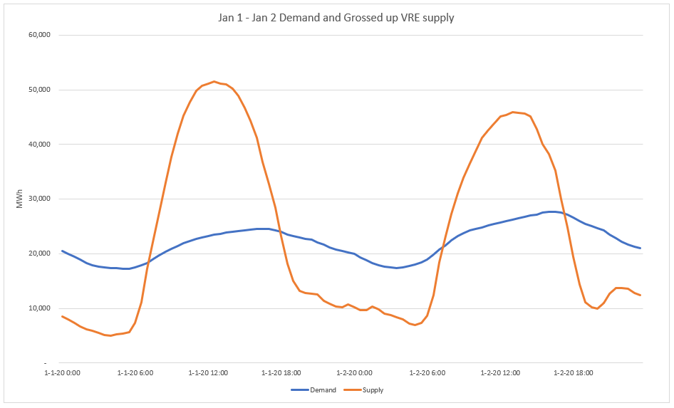
Figure 6 Source: NEMreview

 

Introducing the cumulative deficit (surplus)

So we then calculate a cumulative deficit by taking the deficit or surplus in one half hour and adding it to the next half hour and so on for the full year.

 

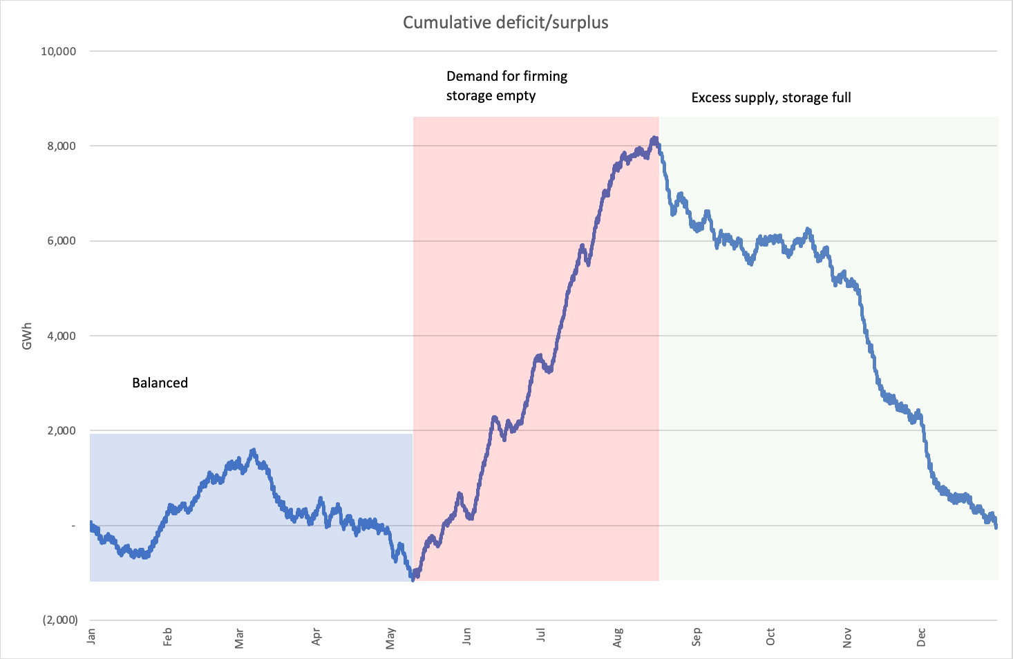
Figure 7 Source: NEMreview

 

The cumulative deficit divides into three periods. A relatively balanced first four months, a large second four month  supply shortfall and a large over supply in the final four months.

Out of interest we can restate Figure 7 into the monthly results, that is the total surplus demand and total surplus generation energy per month:

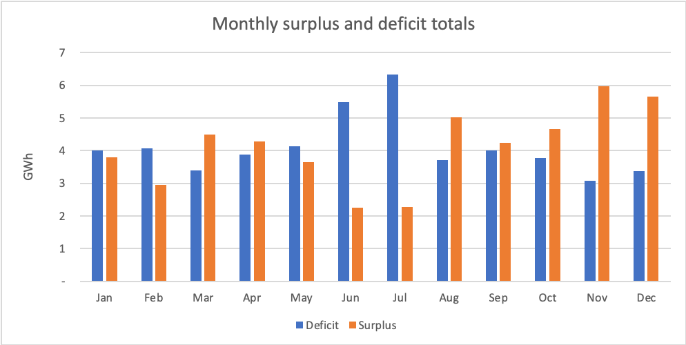
Figure 8 Source: NEMreview

 

In doing this we can more clearly identify at least for this data set that June and July are the big shortfall months and November and December are the big surpluses. Its not just this particular year either. ITK has done quite a bit of work with both simulated half hourly demand, and more optimized supply, and the picture remains broadly similar.

 

How much power and how often

So the Cumulative deficit is an energy deficit over time but we are also interested in how much firming power in Gigawatts is needed at any one time. The next figure shows the percentage of time firming power needed to be X GW or less. We can see that about 85% of the time firming power required is 15 GW or less. A small amount of time, ignored in the rest of this note, up to 27 GW is needed.

 

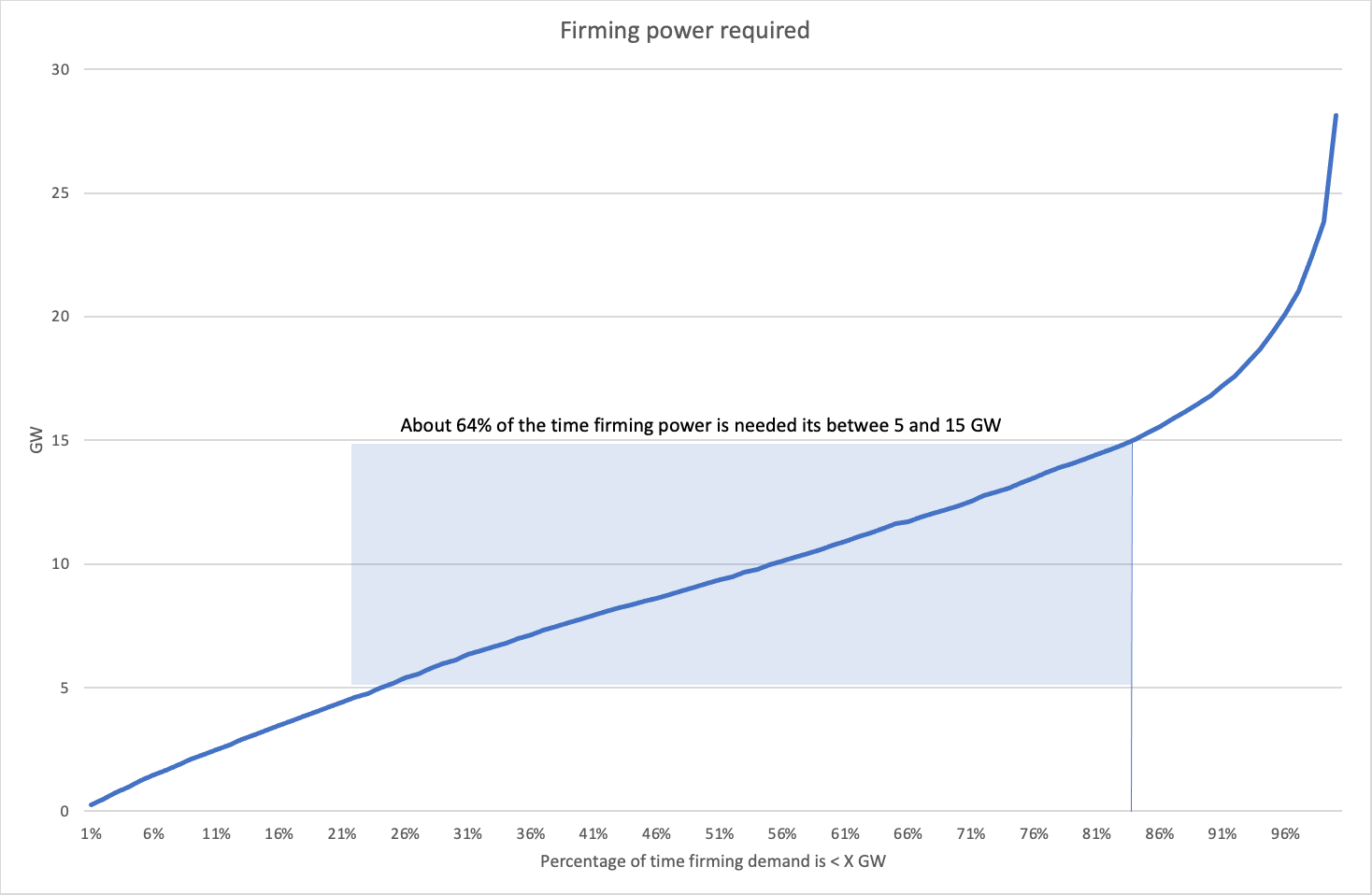
Figure 9 Source: NEMreview

 

What about 15 GW of 10 hour storage?

So the obvious thing to do is to introduce a storage asset. Based on the above figure we used a 15 GW/10 hour asset. It can be a battery or pumped hydro, it doesn’t matter in this study. Round trip efficiency is assumed to be 100%. ITK chose to use 10 hours based on results not reported here. We think the results would be similar if we used 4 hours or 15 hours. At least in this very simple model. When other forms of firming are introduced results can be different, but let’s deal with this simple case first.

The storage asset starts full at midnight on Jan 1 and then as demand exceeds supply in a half hour we match demand and supply using the storage. If supply exceeds demand we put the surplus back into storage.

Since over the whole year total supply is defined to equal total demand then it follows that over the entire year total withdrawals and injections should be equal. Except that isn’t enough because of seasonality. What we find is that about 15% of the time the storage asset is empty when we want it to generate and another 15% of the time its full when we want to charge it.

 

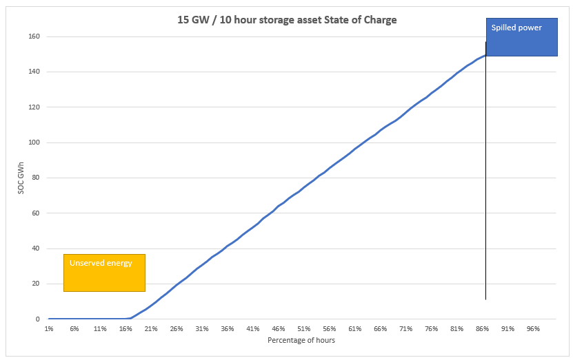
Figure 10 Source: ITK modelling based on NEMreview

 

The combined empty and full hours can be thought of as the unavailability factor.

The next figure shows that there will be times of being empty or being full every single month. In every month there will be unserved and spilled energy.

 

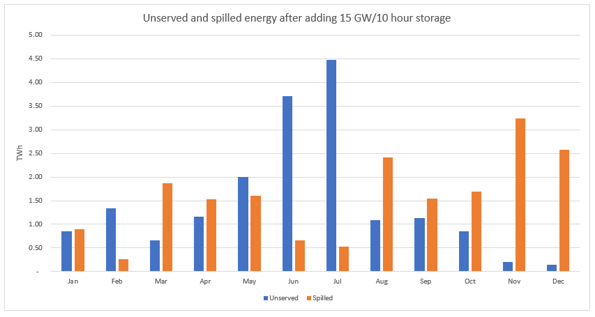
Figure 11 Source: ITK modelling based on NEMreview data

 

It’s a fully decarbonsied NEM with two classes of asset model, not the real world

Of course this is an extreme situation of a fully decarbonized NEM where all the bulk energy is coming from wind and solar. If we relax some assumptions and allow the existing hydro back into the system it starts to solve some of the problems. If there are some gas assets or equivalent around they also help. Demand response (Negawatts) can also do part of the job.

If you don’t like gas then this is where hydrogen might have a role. As noted above hydrogen is expensive to use as electricity fuel and expensive to ship but it is “in the research literature” cheap to store.

There are many, many more wrinkles and with the appropriate market designs, seasonality may eventually be seen as a non-issue.

There is a lot more to be said and this note is mainly intended to represent food for thought.

As we said at the outset though we expect seasonality to show up in the spot market before it shows up anywhere else and we have already seen in 2019 very soft prices leading up to Xmas. So that’s consistent with our theory.

 

——————————————–

About our Guest Author