There’s a few different reasons that I thought it would be useful to share this article today – with some of these being:

1)  The increasing focus we’re devoting to exploration of System Frequency in the NEM – both in terms of:

(a)  Changing longer term patterns of frequency performance:

i.  Which is, at least in part, due to changes in market rules …

>  with the introduction of Fast Frequency Response (FFR) being one example, and

>  the later introduction of Frequency Performance Payments (FPP) being another

ii.  But it’s also to do with the changing plant mix, including:

>  The reduction of the level of inertia in the grid with the progressive closure of coal units; and also

>  The effects of additions of VRE units (especially given that they are operating under Semi-Scheduled arrangements).

(b)  Plus also an increasing number of articles exploring specific frequency disruptions

… which are an increasingly eclectic mix.

2)  But another reason to post this article today is because:

(a)  Earlier this week, I spoke at the NEMdev conference in Brisbane on Wednesday 8th October

(b)  Devoting some of this time to explore some of the recommendations in the draft report from the Nelson Review panel.

(c)  And I’d promised to provide more context on WattClarity … including this article (but more to come, as well).

It’s worth thinking about the effects of imbalance between supply and demand with respect to different time-scales – and, in particular, with respect to these ‘Three of the common building blocks within the National Electricity Market’.

Instantaneous effects, in System Frequency

Starting from first principles (at least for this engineer) my first thoughts gravitate to what happens on an instantaneous basis when Supply ≠ Demand … and that’s an effect that is instantaneously felt (in an AC grid) via the System Frequency.

1)  The smallest building block of data that is commonly available is the 4-second scada data snapshots

… which are now a standard part of of the EMMS since version 5.4, with that change being required for the implementation of Frequency Performance Payments (FPP).

2)  Though we have written an increasing number of articles about our own high(er) speed readings, which sample at 0.1 second cadence

3)  And other readers will point out that frequency disturbances are effectively instantaneous, and propagated through the interconnected network at close to the speed of light.

In earlier articles on WattClarity we’ve used several different images to help illustrate how an imbalanced supply-demand equation impacts on system frequency.

Illustration #1)  Back on 23rd March 2017, Jonathon Dyson wrote the article ‘Let’s talk about FCAS’ … at a time when (>8 years ago) very few people were (how things have changed – which is a good thing!).

In that article, the following animated illustration was used:

Illustration #2)  Then on 6th November 2020 in an article ‘What’s “Primary Frequency Response” and why does it matter anyway?’, Allan O’Neil used the following illustration of a “see-saw”:

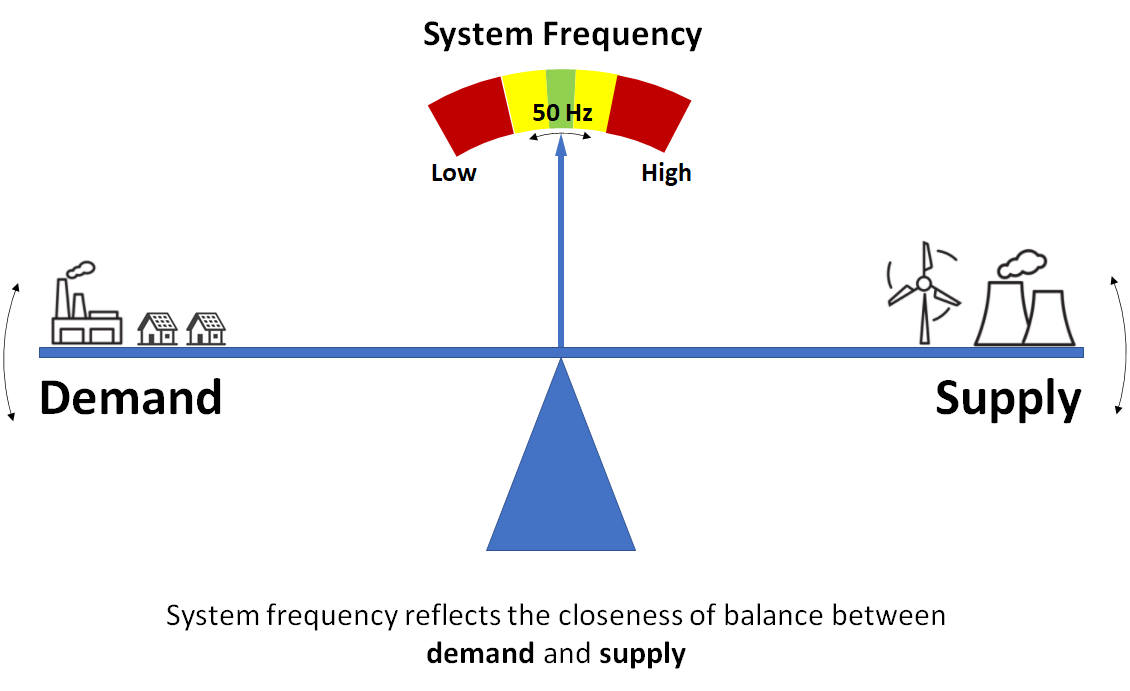
… which Linton then copied into his article ‘About System Frequency’   on 28th February 2025.

Flow on effects, in terms of Economics

The economists on the Nelson Review panel have (understandably) focused more on the Dispatch Interval timeframe, and (whilst noting the challenge of grid stability – i.e. frequency) in my view they focus more on the ‘market efficiency’ sub-optimalities:

To understand where the economic inefficiencies arise, it might be worth refreshing on ‘(A first step into the complexities of) the Dispatch Interval in the Real World’.  With that model in mind, let’s (mentally) step through a few sequential dispatch intervals…

(A)  Let’s consider Dispatch Interval #1

With respect to that article, let’s highlight the following:

1)  at the start of the ‘Magic Happens’ step, there’s a data gathering process to understand the starting state for the dispatch interval

2)  remember (as noted way back in ‘an explainer about electricity demand [take 1]’ ) that the AEMO determines the starting position for ‘visible’ demand served on the grid by adding up supply-side contributions

3)  these numbers are then fed into the AEMO Operational Forecasting processes* to forecast what the level of ‘Market Demand’ is expected to be for the end of the dispatch interval.

* this is an increasingly sophisticated algorithm, which might be explored more in subsequent articles…

4)  This ‘Market Demand’  then feeds into NEMDE, along with Bids and Constraints (plus more) to determine the key outputs – including:

(a)  Targets for all Scheduled and Semi-Scheduled units (and whether the SDC flag is on, or off, for Semi-Scheduled units)

(b)  And also 55 x ENERGY and FCAS prices as well.

5)  Once NEMDE has finished the above:

(a)  Targets are disseminated to all units (received at ~20 seconds into the dispatch interval, which is its own challenge);

(b)  And each unit’s control system sets the trajectory to achieve its Target by the end of the Dispatch Interval:

i.  So this is where we consider ramp rates …

ii.  Remembering that ‘There are actually several different ramp trajectories that are material to dispatch in the NEM’

6)  Through the ~4.5 minutes remaining in the dispatch interval:

(a)  there might be various reasons why the Final Supply does not equal what was forecast to be the ‘Market Demand’  requirement

(b)  so we’ll separately explore these the reasons for this in an article to be later referenced in here.

Through (and at the end of) the dispatch interval, if aggregate supply does not equal to demand – then several responses are triggered:

1)  There are real-time responses as follows:

(a)  The re-enablement of mandatory Primary Frequency Response will have meant that all units (those providing PFR, which should by now be most units) should have* deviated from their targets in the direction required

>> * noting that some may not have, and these might be the unit(s) that triggered the imbalance in the first place.

(b)  In addition, those enabled for Regulation FCAS will have deviated from their Targets by the amount triggered in the AGC 4-second pulses; and

(c)  Less frequently, those enabled for provision of Contingency FCAS might have been required to remotely fire (on the basis of locally monitored frequency) and delivered their contracted response.

2)  But there are also responses at the end of the dispatch interval, feeding into the next dispatch interval.

In terms of cost for this dispatch interval, consider the following two opposite scenarios:

So, no matter whether unders or overs, not consistently nailing Supply=Demand detracts from the Economic Efficiency of the market.

(B)  Now, let’s consider the subsequent Dispatch Intervals

Depending on what the causes might have been for the Supply-vs-Demand imbalance in the earlier dispatch interval, AEMO might (manually or automatically) take certain actions as a result:

1)  such as procuring more Regulation FCAS services:

(a)  if uncertainty about their Demand Forecasts is higher than envisaged.

(b)  or if there is increased uncertainty about supply (from Scheduled and Semi-Scheduled units)

2)  again, the case of 19th August 2025 is an illustrative example (because the AEMO enabled more Lower Regulation Services on that day).

So these factors, together, make it quite important to understand each of the different Types of Events that might trigger supply not equal to demand.