NEMDE nightmares – parallel pathways and clashing constraints

I was recently involved in a training session for users of Global-Roam’s ez2view software where an attendee asked an innocent question about an odd-looking recent price outcome in South Australia. Finding the answer involved descending a fairly deep rabbit hole, but since it’s a good illustration of:

• some of the more complex aspects of the NEM’s dispatch and pricing process, and
• issues arising from the recent energisation of Project EnergyConnect Stage 1 (PEC-1) which has featured in a couple of recent WattClarity posts

we thought it would be worth writing up for those interested.

If you’re not sure what “NEMDE” is, and haven’t grappled in some way with NEM constraints, this probably isn’t the post for you. Otherwise buckle in.

Down the rabbit hole

This was the situation for the 19:05 dispatch interval (DI), NEM time, on Tuesday 11th Feb 2025  as shown in part of ez2view’s NEM Map widget.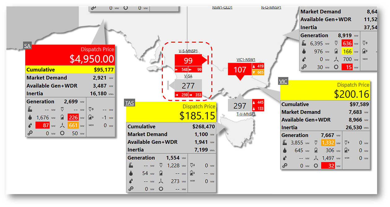

The innocent question: where did the $4,950/MWh price in South Australia (that Paul recorded here earlier) come from?

• A quick scan of bids by our questioner hadn’t identified anyone offering megawatts at that price in South Australia, and
• Aren’t prices set by the most expensive bid dispatched to meet demand?

What are interconnector limits again?

A closer look at the two interconnectors between South Australia and Victoria also raises questions:

• where’s PEC-1?
• On the two links shown, why are the limits on transfers so out of whack?

To explain what this second question’s even about, here’s a blow-up of the interconnector information shown above:

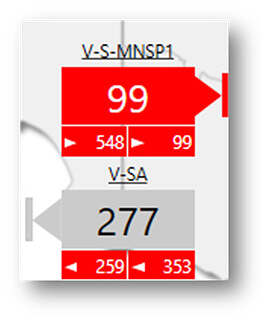
“V-S-MNSP1” is the Murraylink DC cable running from north-west Victoria to mid-north South Australia. “V-SA” is – or looks like – the well-known Heywood interconnector in the far south-west / south-east of the two states.

The large numbers show the target transfer – energy flow in megawatts – across each interconnector, with the icon shape indicating flow direction. The two pairs of smaller numbers with directional arrowheads are (supposedly) the limits on flows when exporting from Victoria to South Australia (on the left) and when importing from South Australia into Victoria (on the right).

Most newcomers to the NEM start with the very reasonable assumption that these flow limits will be something to do with how big the transmission lines and cables between regions are, so shouldn’t differ too much if at all from the inherent physical capacity of these links. Unfortunately that’s often not the case.

So what does set them?

In practice, the limits are very often nothing to do with physical capacity. They are generally set by considerations of system security, or what levels of transfer are possible while keeping all aspects of power system operation robust against disturbances that can inevitably buffet the grid – generators or transmission lines tripping, lightning strikes etc. These limits are dynamically calculated based on the actual state of the power system at any time and can move around a lot.

In this case, these limits are saying that Murraylink can’t import more than the 99 MW it’s carrying into Victoria (this limit is indicated at the bottom right of the icon by the right-facing arrowhead and ‘99’) – sounds reasonable. But at bottom left the Murraylink icon shows that its maximum export to South Australia is -548 MW. That’s negative (indicated by another right-facing arrowhead) 548 MW into South Australia, meaning Murraylink should be flowing at least 548 MW eastwards. This isn’t remotely physically possible, and anyway it completely conflicts with the 99 MW ‘maximum import’ limit.

Things are not much better for V-SA, which has a target flow of 277 MW west from Victoria into South Australia, exceeding an export limit of 259 MW. The graphic also shows an import limit implying that V-SA shouldn’t carry more than -353 MW into Victoria, ie that it should be flowing at least 353 MW westward. Again, in total conflict with the nominal export limit.

After all that time explaining what the limit question is about, I’m not going to answer it here except to say it indicates that the dispatch process was facing great difficulties coming up with a pattern of generation dispatch and inter-regional flows that satisfied all the requirements being placed on it. We’ll see further down what those difficulties were.

Where’s PEC?

Back to the simpler question – where is PEC-1? An actual network map helps here: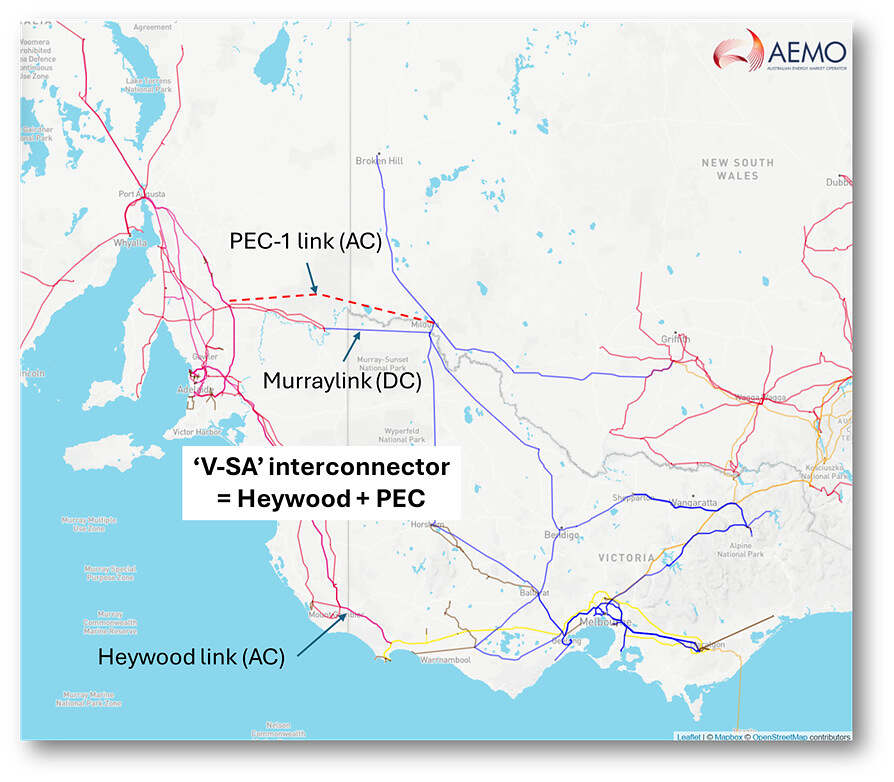

The ‘V-SA’ interconnector used in the market dispatch process now comprises two physical AC links in parallel, the familiar Heywood 500kV/275kV link running through the southwest of Victoria / southeast South Australia, and the new PEC-1 330kV/220kV connection between Bundey in mid-north South Australia and Buronga in NSW which then connects into northwest Victoria via Red Cliffs. Flows across these paths can’t be independently controlled – they follow the simple physics of AC networks. Market dispatch treats the two as a single interconnection whose flow is the sum of physical flows on the two links.

For anyone wondering how two parallel links can be controlled in combination, when neither of them can be individually – good question. They can’t. All the dispatch process can do for AC-connected regions is set targets for controllable generators and loads on either side of their boundary (as well as for controllable DC links like Murraylink). By choosing suitable targets for these controllable elements relative to demand in each region, the process can effectively determine a net AC transfer target across all the pathways linking the two regions. If generators, loads, and DC links all follow their targets exactly (almost never happens), and demand is exactly at the levels forecast (definitely never happens), then the overall AC transfer should be at exactly the planned level. In practice, net variations in supply and demand in adjoining regions play out as variations in the actual inter-regional flows.

At the time of this price event, hot weather meant demand in South Australia was very high (over 2,900 MW) and the Heywood connection was transferring power into South Australia; at the same time high demand in northwest Victoria / southwest NSW, and the lack of solar farm output in these areas at this time of day (20:05 eastern daylight saving time) meant that PEC-1 was carrying power out of South Australia into Victoria. The net V-SA flow (306.6 MW at the start of the interval, available in an ez2view widget I haven’t shown here) was the sum of flow across the two links, with flows out of Victoria to SA positive by convention and flows out of South Australia negative. Market data doesn’t routinely show the split between the two physical links, only the net total. Based on some back-calculations, I’ve estimated that the physical flows at interval start were something like 163 MW eastwards on PEC-1 and 470 MW westwards on Heywood.

Don’t forget system security

Unlike market dispatch, network security limitations – managed through constraints on the dispatch process – needs to respond to and deal with not only combined transfers between regions, but also flow levels on individual physical links. In this interval, one network constraint labelled I_6F_SN_150 was seeking to limit eastward flows on PEC-1 to under 150 MW by interval end. At the same time, other constraints – related to a scheduled outage of one of the two Heywood interconnector circuits due to start at 19:30 – were seeking to reduce the overall AC transfer from Victoria to South Australia (ie the V-SA combined flow across Heywood and PEC-1) to 277 MW or less westwards, again at interval end. At the start of the interval both quantities were outside these secure levels.

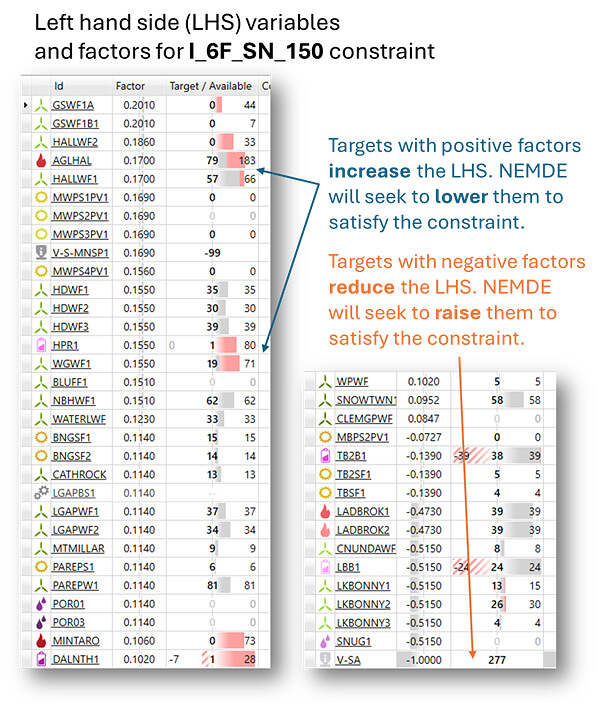
To reduce eastward flows on PEC-1, the dispatch process could seek to increase overall westward transfers from Victoria into South Australia, by increasing the dispatch target for V-SA; alternatively or in addition, it might seek to reduce output targets for South Australian generators (and/or increase charge targets for batteries) relatively close electrically to the PEC-1 connection point, because some of their output naturally tends to flow eastwards across PEC-1. These options are reflected in the target variables and constraint factors (coefficients) present on the left-hand side (LHS) of the I_6F_SN_150 constraint (the screenshot mashup below is from ez2view’s Constraint Equation Dashboard widget):

Help, I’m cornered!

The problem with trying to reduce PEC-1 eastward flows by increasing the target for V-SA flows from its start of interval level (307 MW) is that this would violate one or more of the outage-related constraints limiting its transfers into SA at the end of the interval to 277 MW. So in trying to satisfy the I_6F_SN_150 constraint, the dispatch algorithm (NEMDE) would have to reduce generation in South Australia. In the screenshot above we can see that the LHS targets for several generators and batteries (targets are the bold values in the ‘Target / Available’ column) have indeed been set to levels below their offered availability, shown at the right of the same column.

Target flow on the Murraylink interconnector (which can be independently dispatched by NEMDE because it’s a DC link) have been set to -99 MW, meaning imports into Victoria, because moving power eastward on this link tends to reduce eastward flows on nearby PEC.

But doing too much of all this runs into yet another constraint – supply (including net transfers) and demand still have to balance in South Australia. With net V-SA exports from Victoria to South Australia limited to 277 MW, 99 MW flowing out of the region on Murraylink, and high South Australian demand, it turned out that there was simply not enough available generation in South Australia to both:

• reduce output targets for generators affecting the I_6F_SN_150 constraint by enough to satisfy the constraint (ie bring PEC eastward flows down below 150 MW), and still
• dispatch enough generation in South Australia to meet demand net of transfers on V-SA and Murraylink

NEMDE was being boxed into a corner by competing constraints. How to escape?

The constraint violation escape hatch

When something has to give, the market dispatch design allows constraints to be violated – at a price.

Technically this is accommodated in NEMDE’s linear program by including a “constraint violation surplus” (or “deficit”) variable on the LHS of every constraint. These variables are “hidden” in the sense that we don’t see them in the AEMO MMS constraint coefficient data and hence in tools like ez2view, but they are available to NEMDE to ensure that it can always solve the dispatch optimisation problem and produce a result without giving up because of problem infeasibility. These violation variables typically carry very high penalty prices in the optimisation’s objective function to ensure that they are only set to non-zero values when absolutely necessary.

If none or not all of that last paragraph is comprehensible, all you really need to know is that the dispatch process has a lever called “constraint violation” which it can pull when it encounters clashing constraints.

In this interval, it wasn’t possible to solve the problem and satisfy all constraints without using this escape mechanism. To allow dispatch of enough South Australian generation to balance demand, the constraint violation variable for I_6F_SN_150 had to be set to a non-zero value – visible in ez2view as the “violation degree” for the constraint:

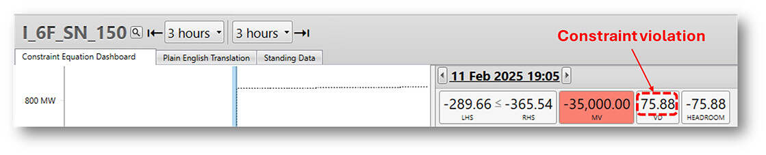
The ordinary target variable values on the constraint’s left-hand side can’t be brought to a level that satisfies the constraint in this interval, hence the odd-looking statement “-289.66 <= -365.54” (which wasn’t mathematically true the last time I checked). The two numbers here are the constraint’s calculated LHS and RHS values for this interval. But if we subtract the constraint violation variable’s value of 75.88 from the LHS we do get -365.54 and see that the constraint is technically satisfied.

For anyone wondering why the RHS is not the secure limit for PEC-1 eastward flows, ie something around ‘150’ – very good question but the way that this type of constraint is formulated means that while the physical limit is strongly involved in the RHS calculation, so are a lot of other quantities, and the resulting number doesn’t have direct physical significance. But if NEMDE can find a solution with LHS <= RHS, that should translate to PEC-1 flows less than the secure limit.

For this particular constraint, the violation variable carries a penalty cost of $35,000/MWh, which is directly reflected in the constraint’s marginal value of -$35,000/MWh. “Marginal value” for a constraint can be defined as the change in NEMDE’s solution cost for a 1 MW increase on the right-hand side (RHS) limit. Since the constraint is in the form LHS <= RHS, increasing the RHS would reduce the constraint violation degree by 1 MW and therefore reduce the solution cost by $35,000/MWh – hence the negative sign on marginal value.

So, back to that spot price

But how on earth do we end up with a South Australian spot price of $4,950/MWh out of all this?

Well, the spot price is by definition the marginal cost of meeting an additional unit of demand in South Australia (not necessarily the highest priced bid dispatched). With no increase in imports from Victoria possible because of the 277 MW V-SA limit, NEMDE would have to increase generation in SA by 1 MW to meet this increase. The screenshot of LHS variables and factors for the I_6F_SN_150 constraint above showed (amongst others) two units, AGLHAL and HALLWF1, with dispatch targets below their offered availabilities. These are the two generators which would receive higher targets for a 1 MW demand increase – we learn this via the Price Setter data for the interval: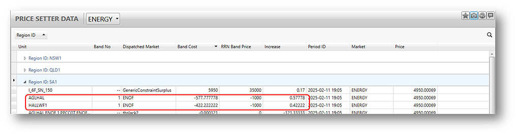

The ‘Increase’ column shows the dispatch target increases, in MW, that would occur if supplying a 1 MW increase in South Australian demand. The values for these two generators, 0.57778 and 0.42222, add to exactly 1: increase in supply = increase in demand. The ‘RRN Band Price’ column shows the marginal generation offer prices for these units, both at -$1,000/MWh. The ‘Band Cost’ column shows the change in NEMDE’s objective function value that would result from these increases – a reduction of $1,000/MWh for a combined 1 MW increase in output, because of their negative offer pricing at -$1,000/MWh.

Constraint balancing

But just above them, we also see a price-setting entry for I_6F_SN_150 with the label ‘GenericConstraintSurplus’, a Band Price of $35,000/MWh, and an Increase of 0.17. This is the impact of the “hidden” constraint violation variable. Why is its ‘Increase’ quantity only 0.17 not 1?

This is because the I_6F_SN_150 constraint factors applying to the two marginal generators, AGLHAL and HALLWF1, are each 0.17, also shown in that earlier constraint dashboard screenshot. When their combined dispatch target increases 1 MW, the constraint LHS value increases by the product of their constraint factor and dispatch target increase: 0.17 x 1 MW = 0.17. This is the amount by which the constraint violation variable therefore needs to increase to balance the constraint (equivalently, this is the increase in constraint violation degree associated with a 1 MW target increase across these two units).

The increase in solution cost associated with this 0.17 marginal increase in violation degree is set by the constraint violation penalty price of $35,000/MWh for I_6F_SN_150, and appears in the ‘Band Cost’ column at $5,950/MWh (ie 0.17 x $35,000/MWh). Different constraints are assigned varying violation penalty costs – violating the #V-SA_RAMP_F constraint which is limiting V-SA overall transfers would cost a whopping $612,500/MWh. This is why the I_6F_SN_150 is the one selected by NEMDE for violation – it’s the cheapest way out of the clashing constraint corner.

Back to that spot price – really

So, finally we can fully answer the very first question that prompted this whole piece – the basis for the spot price? Well, that’s just the overall change in solution cost for meeting the 1 MW change in SA demand. This is just the sum of the contributing band costs including the constraint violation:

• -$1,000/MWh for the additional 1 MW dispatch of AGLHAL and HALLWF1, plus
• $5,950/MWh for the additional cost of violating the I_6F_SN_150 constraint by another 0.17 MW

Totalling $4,950/MWh, the published spot price for the interval.

An obvious question at this point is whether this price has any economic significance? It’s predominantly driven by a constraint violation penalty price of $35,000/MWh which looks almost arbitrary (but noting it’s exactly twice the Market Price Cap of $17,500/MWh), not an actual price offered by any generator(s). If the penalty price had instead been $70,000/MWh, the spot price might have been $10,900/MWh.

It’s certainly true that there is arbitrariness in the specific number, but a high spot price does at least signal that the dispatch process was seeking additional generation, even offered at high prices – if it could have found any that didn’t worsen the violating constraint. Beyond that, it is difficult to assign any greater significance to the published number.

Security might still trump economics

While all the preceding explanation hopefully answers the economic / mathematical reasons for why this spot price came about, the constraint violation means that the power system may not have been in a completely secure state at the end of this interval. (Assessing this would usually require access to physical system measurements we don’t get to see via the MMS.) In simpler terms, PEC-1 flows are probably going to exceed the maximum level the I_6F_SN_150 constraint is trying to allow (by around 20 MW in this case).

A repeating series of constraint violations like this, and underlying data confirming that system security limits are being exceeded, might fairly rapidly require AEMO to intervene in some way, in this case via non-market actions that would somehow reduce flows on the PEC-1 link.

In the event, we did see one further interval involving constraint violation at 19:15 (price set at $5,550/MWh) but that was all, fortunately.

=================================================================================================

About our Guest Author