
Last week saw another eventful couple of days in the NEM, with the NSW region hitting the Administered Price Cap on Wednesday evening, for the first time since the Energy Crisis of 2022.
In the week since then, we’ve fielded various questions about wind farm performance in New South Wales, and the effect of network constraints. Paul began to address this in this first analysis piece here, but this afternoon I wanted to share two visualisations below, which should provide a closer look into the geographic spread of wind conditions and unit availability, and some context about network topology.
The first is from the Bureau of Meteorology. This Mean Sea-Level Pressure (MSLP) chart shows atmospheric pressure. In an MSLP chart, wind strength outside of the tropics is inversely proportional to the distance between isobars i.e. close together lines represent stronger winds.
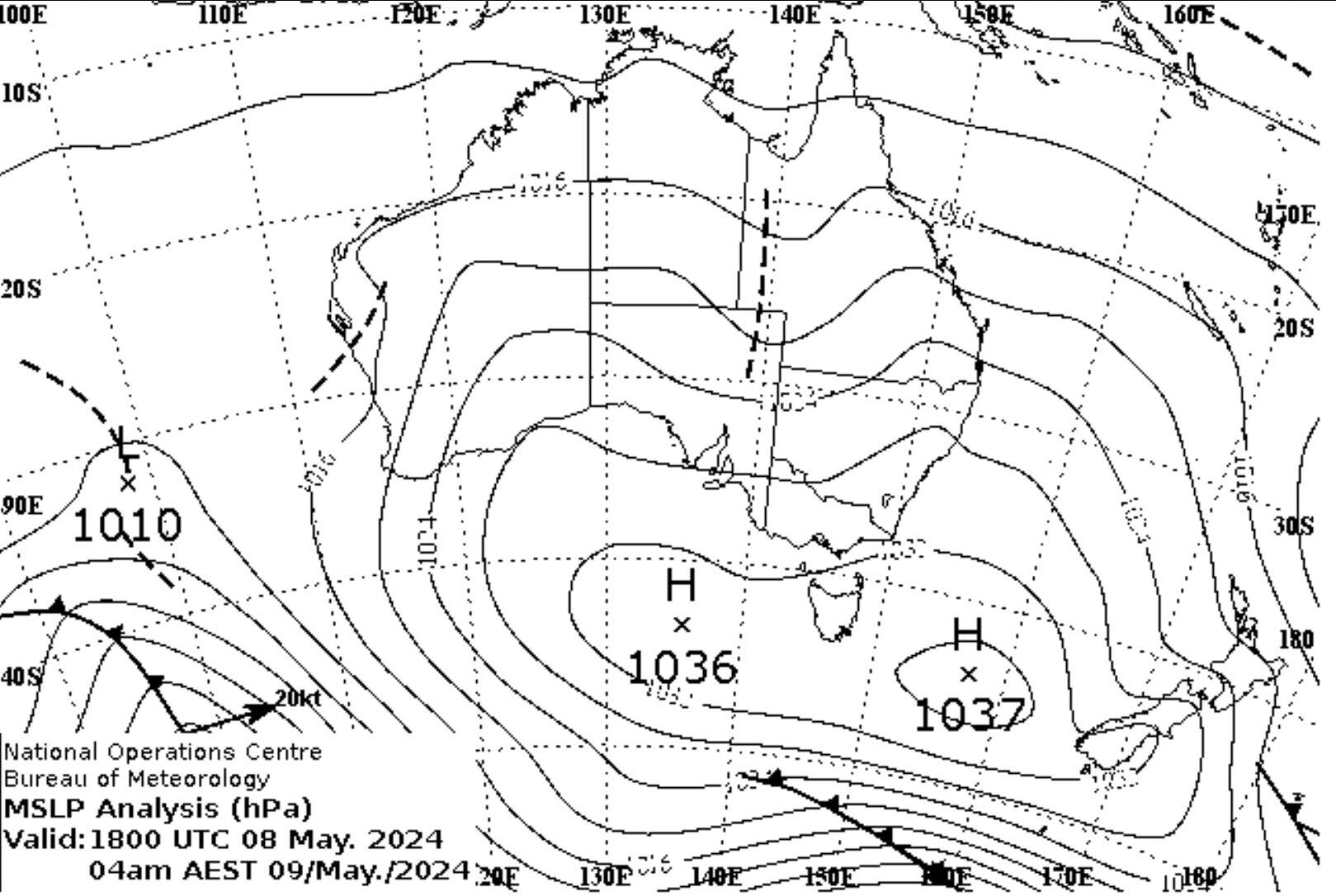
Mean-Sea Level Pressure Analysis for 6pm on Wednesday, 8th May 2024.
Source: BOM
Although not quite as bad as what we saw in the middle of April, the chart above shows high pressure systems over the Southern Ocean, blocking cold fronts from the Antarctic direction. This resulted in below-average wind speeds for much of the eastern half of New South Wales in the early evening on May 8th.
The second chart below is one I’ve compiled using data from our NEMreview software and it shows the relative size of each wind farm (the scaling of each pie chart’s size), and the generation, curtailment and unavailability (coloured slices on each pie chart) for the 18:30 dispatch interval last Wednesday evening.
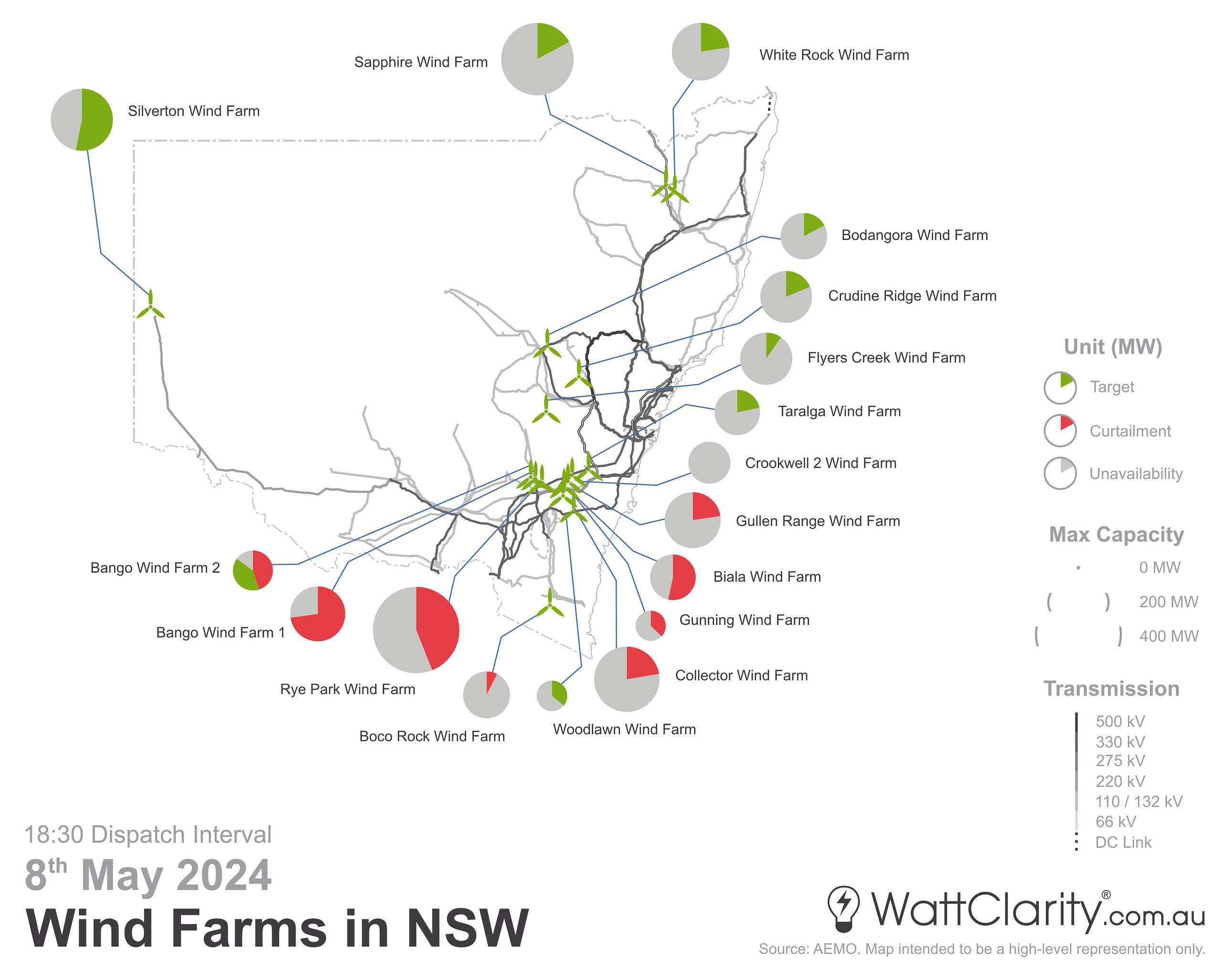
Generation, Curtailment and Unavailability (all in MW) at each wind farm in the New South Wales region last Wednesday for the 18:30 dispatch interval.
Source AEMO, NEMreview
Here on WattClarity, I’ve recently written about curtailment and about our more-detailed methodology for distinguishing between network and economic curtailment. For convenience I will point out the following in relation to the colours in the pie charts in the image above:
- Green is Generation. I’m using that term for simplicity’s sake, but more astute readers should note in the image that I am specifically referring to each unit’s ‘target’ – which differs slightly from the actual metered output of generation.
- Red is Curtailment (of any kind). Given that the spot price in NSW was $14,100/MWh during this interval, there is a strong indication that this was all network curtailment.
- Grey is Unavailability. This is simply the remaining amount of a unit’s capacity (e.g. megawatts below capacity that weren’t generated due to insufficient wind conditions, etc.). You could calculate the Availability by summing together the green and red portions mentioned above.
The visualisation shows that only a handful of wind farms in the region had availability above 50% at this specific point in time.
More notably, there was a significant amount of curtailment occurring in and near the Southern Tablelands region. By firing up my copy of ez2view, I can take a closer look into the constraint equations impacting these wind farms. I specifically note the N::N_CTYS_2 transient stability limit constraint was impacting a number of wind farms – with Collector, Crookwell 2, Gullen Range, Biala, Rye Park and Boco Rock all appearing with high factors on the LHS in this constraint equation. Paul has already written a longer piece covering this constraint equation.
There are almost guaranteed to be other factors at play (interconnector limits, other constraints, etc.) but that is all I have time for late on a Friday afternoon. As time permits we hope to follow this up with further examination.
Not quite sure I understand the logic here. The so-called network curtailment is almost irrelevant. It was never 100% of the wind farm capacity. You can only curtail something if it was capable of generating anyhow and none of the “Southern Tablelands were producing anything. If there was any wind they would look like (say) Bango Wind Farm #2. Touching a transient stability limit probably just implies the transmission network was getting full with Thermal and Hydro MW to keep the lights on and would no longer be N-1 fault tolerant for significantly more coming from this region.
Hi Andrew, the second chart is meant to show that the wind conditions for the wind farms in the Southern half of the state were still generally better than for those in the North-East – but NEMDE was constraining those wind farms down (to 0MW except for Bango Wind Farm 2) largely because of the N::N_CTYS_2 constraint equation.
As mentioned in the article, Green + Red = Availability and Grey = Unavailability.