
As we have seen from previous posts, the NEM is a complex place. With the benefit of hindsight, a number of these factors become quite clear. Sometimes, seeing things in hindsight is not enough and foresight is needed.
Specifically the post will look at hedge levels. Hedge levels will, to a large extend, define bidding behaviour unless there are physical issues with the plant. In my experience, the prime motivation for a generator is to have the prices as high as possible if they are generating above their contract position. This is also known as the price/volume trade off as generators can be in a situation where reducing their expected output (volume) could increase price (or vice versa).
This price/volume trade-off usually involves covering contracts as long as the prices in the spot market are above the cost of production (short run marginal cost – SRMC). If the price is below SRMC, it is cheaper to buy from the spot market than generate. Above their contract levels they will usually try and achieve as high a price as possible while generating as much as possible. If they cannot meet their contract levels, they will want to have the price as low as possible. In order to estimate SRMC I used the report from ACIL Tasman which is publicly available.
Structure of Contracts
The contract position can be different from one half hour to the next and will be made up of different products.
The standard contracts have peak periods (7:30 to 22:00 on working week days) and non-peak periods (all other periods). These are the most traded contracts but counterparties are free to agree any period(s).
Usually the contracts are annual or quarterly. This means that the position typically changes with the calendar quarter.
The contract doesn’t have to perfectly cover the spot price. If a participant only wants to cover itself when the price is above a certain threshold (usually $300/MWh) they can purchase a cap contract. This is usually purchased by retailers to protect themselves against coincidences of price increasing while their demand increases or as an alternative to purchasing a standard contract.
The hedge levels are typically estimated for an entire corporation as they will not typically hedge units individually.
Where a corporation (such as AGL, Origin, or EnergyAustralia) has interests across more than one region, my experience has shown that they will be trying to cover their contracts using an assumed probability of price separation. It is difficult to estimate what this assumed price separation is but it is a necessary step to estimate the hedge levels for these corporations.
For simplicity, I have looked at CS Energy which has its main interests and all generating assets in Queensland. CS Energy also has a large portfolio of generating units which means that their aggregated bidding is less sensitive to individual plant issues. Finally, I am most familiar with the Queensland market which makes it slightly easier for me to pick a good portfolio here.
Another feature to remember is that contract positions can change during the period so even if you have understood the behaviour of a participant, the contract position may change. This would then require fresh analysis to understand the new behaviour.
Example of estimated contract position
To illustrate how we can estimate a contract position I have looked at CS Energy’s bids in the first calendar quarter of 2013 (January to March).
In order to estimate both peak and off-peak behaviour I will ignore the first of January (as public holidays only have off-peak periods).
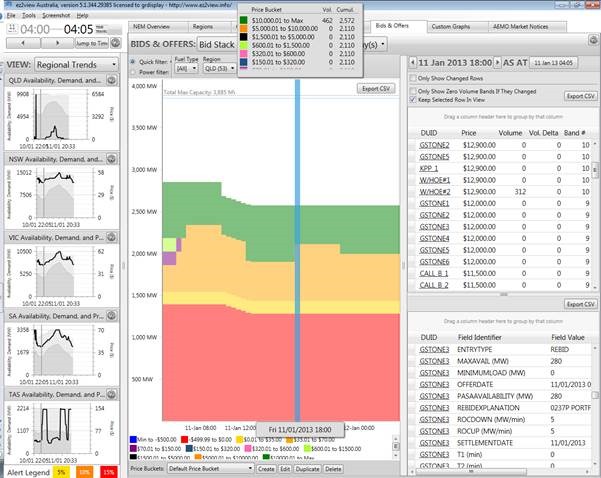
Below is a view of 2 January 2013 as seen through Ez2View’s Time Travel function.
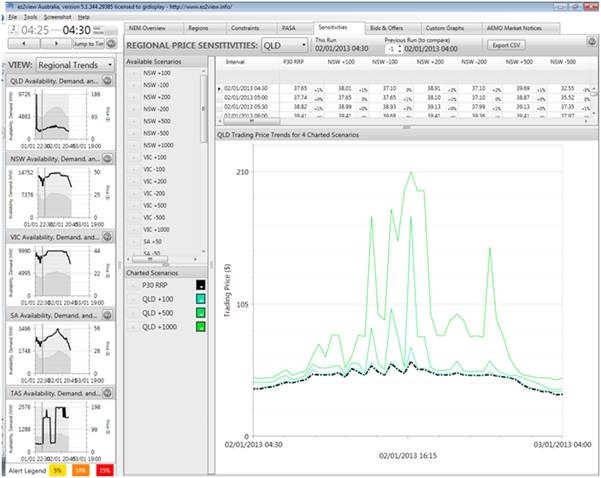
The price estimation in pre-dispatch was not surprising given the time of year. Even if demand was underestimated by 1,000 MW by the pre-dispatch run (‘QLD +1,000’ line above) the price was not expected to go above $210/MWh.
The default bid (daily bid) of CS Energy for the day is published by AEMO the next day at 4:00. An analyst can use this to determine likely hedge levels.
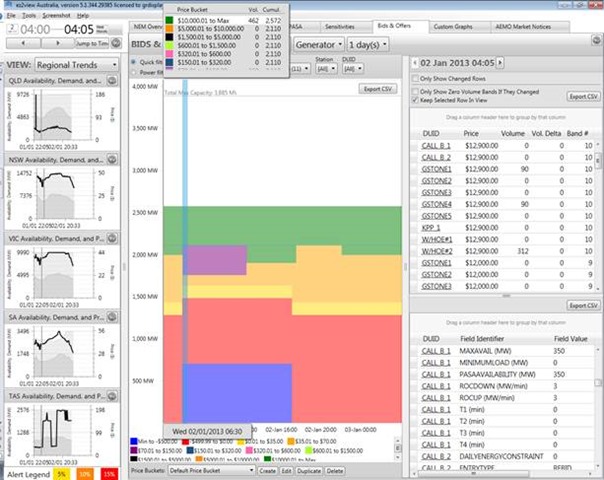
The top left corner shows that this was the view at 4:05 which is the start of a trading day.
The blue and red blocs are bids below $0/MWh. This is the minimum generation that CS Energy wants its plant to produce. The reason why they are willing to potentially pay to generate is to make sure that its coal fired generation doesn’t get turned off as re-starting is expensive. The yellow line is just below the SRMC of its cheapest plant (Kogan Creek) when accounting for the added expense of carbon.
The most interesting bands are the orange and purple. The purple band represents generation at a strategic price. This price includes the SRMC but also a contribution towards long run costs. It would be cheaper for CS Energy to generate at this level than purchase from the spot market so it is most likely the band they want to use for price/volume trade-off.
The orange band is the SRMC of its base loading plant. As they have available generation above this level, it is likely to represent the hedge level. There are three distinct patterns.
1) Midnight to 6:30 (highlighted area) and from 22:00 onwards
2) 6:30 to 18:00
3) 18:00 to 22:00
These are likely to represent the three different stages of hedges. Stage one is the off-peak hedges. They have a total bid of 1,990 MW at this level which is exactly the same during all off-peak periods. Though off-peak doesn’t end until 7:30, CS Energy has rebid from before that time in order to make sure that by 7:30 they are actually generating to their hedge levels instead of ramping up towards it. The other risk in the morning is plant tripping off as they try to ramp. This could cause price spikes which CS Energy would want to be capturing. The rest of the generation is bid in (green line) at very high prices (above $10,000/MWh). There is no volume between $51.85/MWh and $12,900/MWh which means that if the price is higher than SRMC, CS Energy’s default position is to let the price go to the market price cap.
The second period is 6:30 to 18:00. There is around 1,750 MW bid at SRMC with an additional 360 MW only available if prices get above $90.01/MWh.
The last period is from 18:00 to 22:00. There is a distinct increase of 210 MW in available generation at SRMC prices during this period.
My theory is that CS Energy had sold 1,990 MW of off-peak swaps, 1,900 MW of peak swaps and an additional 200 MW of swaps from 18:00 to 22:00 (evening peak).
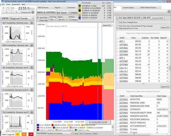
When the bids are published we can also Time Travel to the end of the day to see how their final bids turned out.
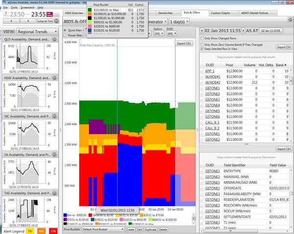
During the day there was some strategic bidding and some plant issues. This resulted in a lot more generation offered below -$500/MWh to avoid being turned off.
The purple band now looks much more erratic. During the day, CS was willing to put the volume in this band into the high priced green band in order to try and get the price higher. The other bands have been largely kept the same which makes my conclusion more plausible.
Confirming the Assumptions
Though it is not possible to truly know the contracting position of a portfolio, the conclusions above can be tested during a more volatile period.
During summer there were a number of volatile periods. Below is 11 January as it would have looked to the spot traders at 4:05 that morning.
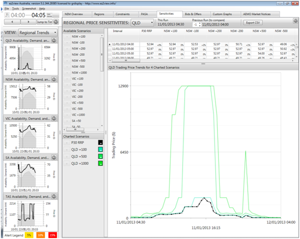
The price was estimated by pre-dispatch to be well above the cost of generation. It is also noted that even the +500 sensitivity had prices at $12,900/MWh for a large part of the day. Incidentally, we posted a short view at the time of the high demand seen on the day.
The initial bids from CS Energy indicate that the conclusions above are likely to be correct.
The gradual step down at the start of the day is Gladstone unit 1 coming offline for a scheduled outage. There is additional generation bid in during this time which is likely to make sure that the portfolio can meet its obligation even if Gladstone unit 1 trips as it ramps down. Another alternative would be that the prices in pre-dispatch are much higher than SRMC and CS Energy believe they can generate without reducing the price.
Other than the issue with Gladstone unit 1 coming offline, the bids show the same three distinct bid periods as seen on 2 January. The sensitivities mean that the purple block has been replaced by a lower priced orange so that CS Energy’s default position is to generate during the high prices.
The block from 18:00 to 22:00 is still there at a time when the sensitivities (prices in graph above) are reducing. If CS Energy wasn’t contracted, it would be undesirable for them to generate during this time as they act to suppress the price.
The final bids were similar to the initial ones. Once again, more generation was offered below -$500/MWh to stay dispatched but looking at the three block of time from above, the desired generation level stayed the same. Note that the block from 18:00 to 22:00 changed to higher prices but only when CS Energy was confident that they would still be dispatched.
The conclusions from 2 January still hold. In practice the analysts would continuously monitor bids and output but to a more casual observer this is likely to be the hedge level of CS Energy during the quarter.
There is more analysis conducted. This includes looking at exactly what prices a portfolio is willing to generate less and how sensitive the portfolio is to different price levels to determine cap cover.
Remember: hedge levels can change during the quarter, which makes it important to continuously monitor behaviour if relying on the estimates.
Validity of Initial Bids
Using initial bids is good for analysis because the bids tend to be using more of the portfolios own knowledge and rely less on prices and short term forecasts.
As mentioned above, the period from 18:00 to 22:00 ended up with a number of periods bid in well above SRMC. This was done at a time when CS Energy was confident that they would be dispatched and, as we saw, they changed their bids as the sensitivities changed.
The question then becomes how realistic the initial bids are. The Australian Energy Regulator has set out a principle that all bids (and re-bids) must be made in Good Faith. This means that a generator, in the absence of new information, must intend to honour the bid when it was made. This means that a generator cannot put in a bid to ‘confuse’ or hide its intention.
Why Estimates Hedge Levels
The most common use of estimated hedge levels is by spot traders. They have to estimate the market impact of their decisions which includes how other would react. Some spot traders will literally spend hours each day analysing and monitoring bid behaviour. They have to get their daily bids submitted to AEMO by 12:30 the day before the trading day. This gives them from 4:00 to 12:30 to analyse the previous day’s bidding before submitting their own for the next day. After 12:30 the day before the trading day, the price bands for the bids cannot be changed. The volume (and other technical parameters such as availability and ramp rates) can still be changed but only if there is a material change in conditions.
The other group is the financial analysts. Patterns emerge over a period of time which can be used for medium (up to 12 months) and longer term analysis (up to five years). It is more the interrelationship between previous market conditions (spot prices, hedge prices etc) and current hedge levels which are inferred by the financial analysts. These forecasts often feed into budgets and risk parameters.
Derivative pricing (performed by derivative traders or analysts) is often done based in expectation of spot prices in the short term. A key factor of spot pricing is the hedge levels of the generators. Traders can also use the current hedge levels to infer what the desired future hedge levels would be for counterparties. This could give them an advantage in negotiations if they believe that their counterparty needs a lot more hedges in a short amount of time.
About the Author.
Thomas Dargue has worked with both private and publicly owned generators as well as for Ergon Energy over the last seven years.
Feel free to posts comment on this page or email directly to Thomas@global-roam.com. He is also on LinkedIn
.
Editor’s Note: Pre-Order your copy of our QLD Market Review before 24th May and save
Our detailed review of what happened in Queensland over summer (and into Q1), that Thomas has been heavily involved in preparing, will be released at the end of May.
For those who want to have their copy delivered as soon as it is released, you can pre-order today and save 16%. Just fax back this order form (an offer just for WattClarity® Readers) with your details.
Be the first to comment on "Estimating Hedge Levels"