
As noted here, for every DUID that operated at some point through CAL2019, we include two pages of statistical data on the technical and commercial operations of the plant:
![]()
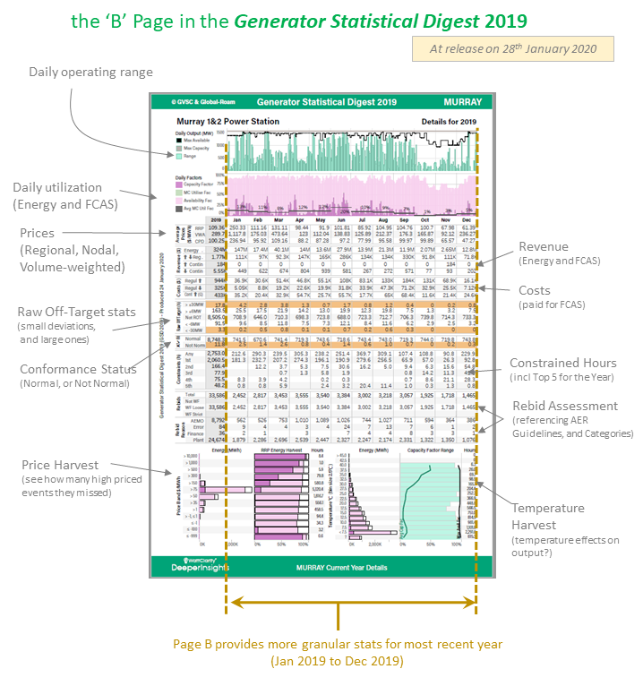
We’re referring to the page on the left as the ‘A’ Page (described here), and the page on the right as the ‘B’ Page (which is described below).
In the table below, we provide more context to the data represented on each ‘B’ Page in the GSD2019:
| Data Sets Included | Brief Description |
| Daily Operating Range | Through 2019 we witnessed (and were involved in) some discussions with a broader group of energy sector stakeholders about the ‘typical’ operational patterns of different types of power generation assets – particularly as the market is likely to be requiring more flexibility in future years.
The addition of the ‘B’ Page into the GSD2019 provided the ideal opportunity to start the page with this simple trend that will help readers to quickly understand the operational profile of the unit in question – and, by comparing page-to-page, contrasting these operational profiles. |
| Daily Utilisation (for Energy and FCAS) |
As a ready-reference guide to assist in understanding, and communication, of operational patterns of the DUIDs operational across the NEM through 2019 we include the Daily Utilisation chart.
An increasing number of assets (particularly batteries) will be added to the grid in the coming years with a focus not just on Energy but also on the provision of FCAS services. With these assets, it’s important to recognise that “utilisation” – hence the adoption of metrics that span commodities: |
| Prices (Regional, Nodal and Volume-Weighted) |
Three different monthly prices are provided for the unit in question:
Data Point #1 = Monthly Time-Weighted Average (TWA) spot price for the region containing that DUID are included in the table as a point of comparison. Data Point #2 = Volume-Weighted Average (VWA) price ($/MWh) for the month for that DUID. The VWA Revenue is a more commonly used metric, which incorporates the effect of the MLF on a generator’s revenue – but readers need to be clear that it’s not the same as VWA Price, which has its own applications (e.g. it has value in comparability between units that does not include the complicating impact of MLF). Data Point #3 = Connection Point Dispatch Price ($/MWh) – which is calculated by AEMO for every dispatch interval and for which we aggregate on a time-weighted basis for each month in the GSD2020 to help the reader understand the impact of transmission congestion on that asset. —————- In particular, Allan’s article ‘How good is Solar Farming?’ on 28th January 2020 highlights how this table in the GSD2019 makes it easy to quickly compare across a broad number of units to understand both: The way in which the GSD2019 makes it easier to understand congestion risk (and impact) was also picked up by Ben Willacy in ‘What lies ahead for the NEM in 2020? Some lessons from 2019’ on 28th January 2020. In his article ‘Highlights from the 2020 GSD’ on 1st Feb 2021, David Leitch drew some useful comparisons between VWA Prices for calendar 2020 from the GSD2020. |
| Revenue (Energy and FCAS) |
Revenue is calculated on a monthly basis through 2019 for each of 4 categories as applicable:
1) Energy for production sent out (i.e. net of approximated auxiliary energy consumption); and also 2) FCAS Regulation (Raise and Lower) 3) FCAS Contingency Raise 4) FCAS Contingency Lower. Because we calculate costs for each just below this, it’s very easy to compare! —————- When we have time, will link in WattClarity articles that have been developed |
| Costs (for FCAS) |
Utilising a methodology that has been developed by Greenview Strategic Consulting (based on understanding of AEMO’s processes) it has been possible to derive the apportionment of FCAS costs (global, and regional) across all Participants (and hence DUIDs), under these three categories:
1) FCAS Regulation (Raise and Lower) apportioned using the ‘Causer Pays’ method 2) FCAS Contingency Raise, apportioned to Generators; and 3) FCAS Contingency Lower, apportioned to Loads. —————- Allan’s article also highlighted the large FCAS costs incurred by some solar farms (and they were not the only ones!) due in part to poor Raw Off-Target performance. In this article (to come) Jonathon Dyson… |
| Raw Off-Target stats | In the GSD2019 we built on what we had done from the GRC2018 (and also incorporated into our ez2view software through 2019) to incorporate a tabular summary of ‘Raw Off-Target‘ performance for each unit.
———- Summary results from the GSD2019 were utilised in publishing a comparative performance list across all Scheduled and Semi-Scheduled in ‘Review of extremes in Raw Off-Target performance through 2019‘. The article highlighted the ‘worst’ performers in each fuel type, and will be followed up by subsequent articles.
|
| Calculated Conformance Status | This ‘Raw Off-Target’ metric is then developed further to derive a ‘Conformance Status’ for each DUID across all Dispatch Intervals in 2019:
1st Category = ‘Normal’, which is where all DUIDs are expected to operate, as part of their registration process. 2nd Category = ‘Not Normal’, which is an aggregation of all dispatch intervals for that unit where a unit was deduced as operating ‘Off-Target’ (according to AEMO’s Compliance logic) and ‘Non-Conforming’ ———- These stats will be utilised in articles on WattClarity from time to time. When we remember to, we will link those articles in here. |
| Constrained Hours | In the longer 10-year trend of annual summary of constrained hours on the ‘A’ Page we list a ‘top 5’ constraints for a DUID through 2019.
On the ‘B’ Page here we expand on those top 5 constraints to record how many hours in each month the constraint was bound affecting that unit. ———- These stats will be utilised in articles on WattClarity from time to time. When we remember to, we will link those articles in here. |
| Rebids “Not Well Formed” | The AER is responsible for issuing Bidding Guidelines, which they expect to be adhered to (as they play an important role in ensuring that participants follow the NEM Rules when operating in the market).
———- In the GRC2018 we included several pages of analysis of bidding (discussed here), drawing on the guidelines to firstly automatically tag each bid as either: This analysis has been extended in the GSD2019, and documented for each individual unit. |
| Rebid Categories | Following on from the initial categorisation, all rebids that could be determined as ‘Well Formed’ were then unbundled into one of the 4 categories prescribed by the AER in its Guidelines:
Category “P” for Plant Reasons ———- When we publish articles using these statistics (and we remember) we will link them in here. |
| Price Harvest | In this figure, we match the output in a dispatch interval with what the dispatch price was for that region at the same time. This presents a great way of helping the reader to understand how well the DUID is maximising revenue opportunities – particularly: (a) Securing the high-priced events; and (b) Avoiding the negatively priced events. ———- On 28th Jan 2020 with respect to the GSD2019, Allan’s article ‘How good is Solar Farming?’ was able to utilise the respective Price Harvest charts to highlight a key difference (in revenue performance) between Solar Farms and Peaking generators. On 1st Feb 2021 with respect to the GSD2020, Marcelle wrote about ‘Using the GSD2020 to explore operating patterns across generation types’ – and this provides an excellent practical guide for how to interpret this element of the annual Generator Statistical Digest. |
| Temperature Harvest | In this figure, we match the range of output at the particular DUID at the ambient temperature recorded at the nearest BOM measurement station (identified at the top of the ‘A’ Page).
———- In ‘Extreme temperature effects on generation supply technology’ on 11th February 2020 we were able to utilise the detailed per-unit analysis published in the GSD2019 to help explore limitations at high temperatures. |
The advantage of this format is that it enables data to be reported, on the same basis, for all 304 DUIDs!