

A quick note on some odd-looking inter-regional flows on Sunday morning (4th October 2026), illustrating how the addition of the new PEC interconnector (NSW1-SA1), along with some familiar constraints in southern NSW, can lead to counter-intuitive (or at least counter-price) energy transfers.
Here’s a NEM dispatch overview for the 09:20 (AEST) interval:

In the three central regions highlighted, every inter-regional link is flowing counter-price:
- 135 MW scheduled westwards on PEC, from a NSW price of $11.88/MWh into SA at $0.50/MWh
- 267 MW scheduled southwards on VNI, from $11.88/MWh to $2.10/MWh
- 303 MW and 143 MW scheduled westwards on Heywood and Murraylink respectively, from $2.10 to $0.50/MWh
All these flows seem to be losing money, not moving energy from lower- to higher-priced regions – why?
Constraints, yet again
Starting with PEC, the interconnector dashboard widget in ez2view shows that it’s subject to three binding constraints:
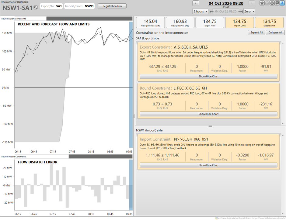
In the export direction (into SA), these constraints are:
- V_S_6CGH_SA_UFLS – this limits total AC flows into SA (on PEC as well as Heywood, although the description only mentions the latter), to ensure that if there is an unexpected interconnector trip, it’s from a flow level low enough for under-frequency load shedding in South Australia to handle without a system collapse. Seems prudent.
- L_PEC_X_6C_6G_6H – this is a version of the new loop constraint associated with the introduction of PEC, which forms a three-state AC loop with the Heywood (Vic to SA) and VNI (Vic to NSW) interconnections. Flow relationships on such loops conform to the laws of AC power system physics. The loop constraint is a simplified representation that aims to keep market dispatch and scheduled flows consistent with these laws.
On the import side, there’s one binding constraint:
- N>>6CGH_060_051 – this is a PEC-aware version of a long-standing constraint associated with transmission bottlenecks between southern NSW and the rest of the state. While it’s nominally a constraint on PEC imports into NSW, we can see that the limit is currently forcing exports of 134.75 MW. (This constraint is also driving Murraylink’s flows out of Victoria, because Murraylink is electrically close to the congested area.)
What’s happening here is that the N>>6CGH_060_051 constraint is forcing these flows to maximise dispatch of cheaply-offered solar and wind generation in southern NSW and north-western Victoria. The magnitude of export flow on PEC is limited principally by the V_S_6CGH_SA_UFLS constraint.
Unpicking the loop
Let’s look more closely at the third constraint involved – L_PEC_X_6C_6G_6H:
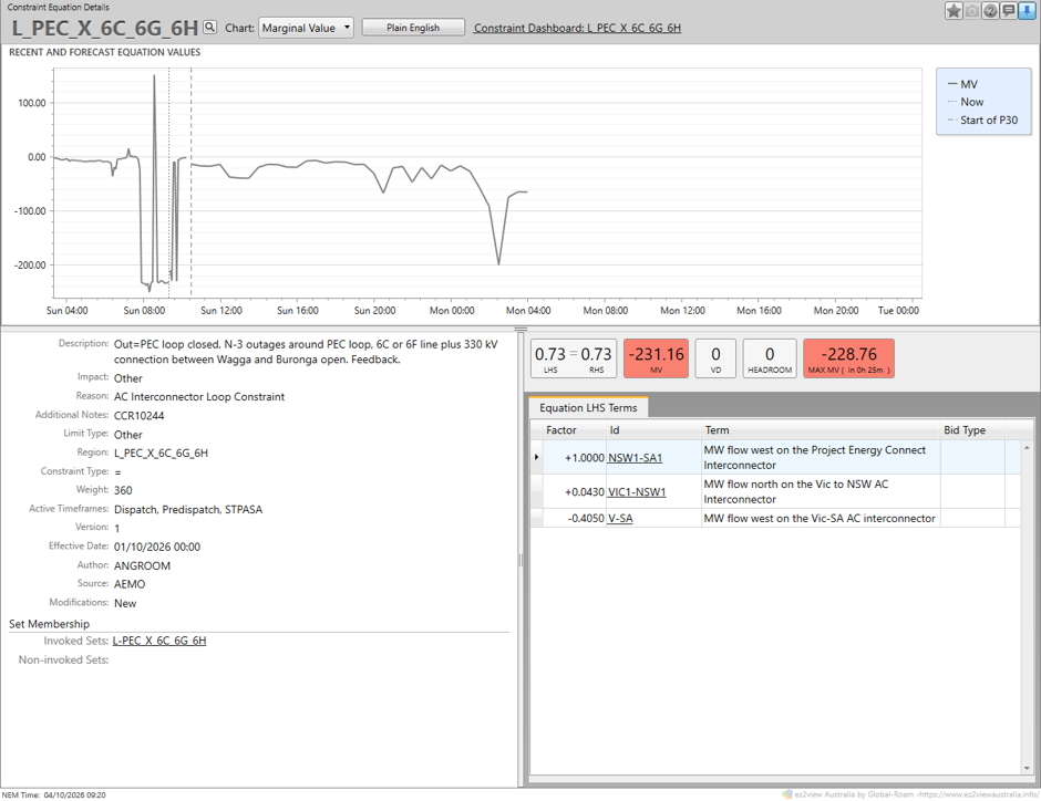
The panel at lower right shows that the constraint involves just the three loop interconnections: PEC (NSW1-SA1) with a factor of +1.0000, VNI (VIC1-NSW1) with factor 0.0430, and Heywood (V-SA) with factor -0.4050.
As we’ve explained elsewhere on WattClarity, this notation translates to the constraint requiring that in any given dispatch interval the flow targets for these interconnectors adhere to an equality relationship:
+1.000 x PEC target + 0.0430 x VNI target – 0.4050 x Heywood target = RHS value
We won’t worry now about where the RHS value comes from – it’s just a given for our current purposes. (But note it can and does change from dispatch interval to dispatch interval – driven by real-time SCADA measurements of power system flows).
Examining the signs and sizes of the factors applying to each interconnector, this equation implies that if PEC target flows were to increase by 1 MW, then to maintain a constant left-hand side value and satisfy the constraint equation, the dispatch algorithm NEMDE would need to make offsetting changes to one or both of the other interconnector targets:
- VNI flows could be changed by -1/0.043 = -23.26 MW, or
- Heywood flows could be changed by 1/0.405 = +2.47 MW, or
- Some combination of VNI and Heywood changes could be made as long as they added up to an equivalent offsetting effect.
So if NEMDE is seeking to increase westward flows on PEC in any interval – due to a constraint like N>>6CGH_060_051 – then because of the loop constraint it will need to make adjustments like:
- On VNI, reducing northward flows, or increasing southward flows – either of which represent negative changes
- On Heywood, increasing westward, or decreasing eastward flows – both positive changes
This all gives us some clue as to why we’ve ended up with:
- Westward flows on PEC – driven by the underlying N>>6CGH_060_051 constraint and NEMDE’s objective of maximising output from cheaply-offered generation
- Southward (negative) flows on VNI and westward (positive) flows on Heywood, both of which help with balancing the loop constraint
But those prices?
Above we’ve established some directional factors driving the loop interconnector outcomes, but to understand why the flows are from higher to lower spot prices we can use constraint marginal values to get some quantitative results that further illustrate what these constraints are doing.
Going back to the PEC overview screen from ez2view, with some key data highlighted:
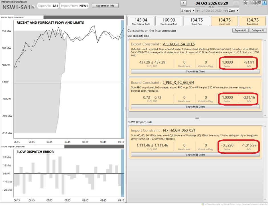
The underlying “forcing” constraint, N>>6CGH_060_051, has a marginal value (MV) of -$1,016.97/MWh, and PEC’s factor in that constraint is -0.329.
We can combine these two numbers to deduce that an additional 1 MW flow west on PEC would benefit NEMDE’s cost function by:
-0.329 x (-$1,016.97/MWh) = +$334.58/MWh
This is what a large ‘marginal value’ means – a small change in the constraint can make a large difference to the total costs that NEMDE is set up to minimise.
But on the export side, that 1 MW extra flow westward would carry costs related to the other two binding constraints: V_S_6CGH_SA_UFLS and the loop constraint, both of which feature PEC with a factor of +1.0000 and also have material marginal values:
+1.0000 x (-$91.91/MWh) + 1.0000 x (-$231.16/MWh) = -$323.07/MWh
Combining these results, it looks like the net benefit of flowing another 1 MW westward would be:
+$334.58/MWh – $323.07/MWh = +$11.51/MWh
But that calculation ignores the loss on the spot price difference for energy delivered to SA out of NSW:
$0.50/MWh – $11.88/MWh = -$11.38/MWh
Not quite balanced (we’re ignoring the cost of interconnector losses) but close enough to show why NEMDE has landed where it has. The spot price difference combined with constraint costs and benefits all neatly balance out. NEMDE can’t improve things by changing PEC flows any further.
Around the loop again
We can apply the same marginal value analysis to Heywood and VNI.
On Heywood, the two binding constraints are V_S_6CGH_SA_UFLS, marginal value -$91.91/MWh with Heywood’s factor +1.0000, and L_PEC_X_6C_6G_6H with marginal value -$231.16/MWh and Heywood factor -0.4050. The opposite signs on Heywood’s factors mean that the constraint values tend to offset each other for a change in Heywood flows.
The net constraint value of an additional 1 MW of westward flow on Heywood is:
+1.000 x (-$91.91/MWh) -0.4050 x (-$231.16/MWh) = -$91.91/MWh + $93.62/MWh = $1.71/MWh
But the spot price difference on that westward flow is
$0.50/MWh – $2.10/MWh = -$1.60/MWh
Again, (almost) balancing out the net constraint value and spot price difference.
Finally, the only binding constraint on VNI is the loop constraint with marginal value -$231.16/MWh and VNI factor +0.0430. An additional 1 MW of southward flow (represented by -1 MW given the flow sign convention for this interconnector) has a constraint value of
-1 x (+0.0430) x (-$231.16/MWh) = $9.94/MWh
Which again closely balances the price difference on that southward flow of:
$2.10/MWh – $11.88/MWh = -$9.78/MWh
Experienced readers will know, in keeping with the “loopy” theme here, that there is a degree of circularity between constraint marginal values and spot prices, so the analysis above doesn’t fully explain the absolute levels of spot prices in each region.
But hopefully it provides some insight into how the new loop constraint interacts with others, when flows on one leg of the loop are being forced by a separate underlying constraint like the one active in this case.
=================================================================================================
About our Guest Author
 |
Allan O’Neil has worked in Australia’s wholesale energy markets since their creation in the mid-1990’s, in trading, risk management, forecasting and analytical roles with major NEM electricity and gas retail and generation companies.
He is now an independent energy markets consultant, working with clients on projects across a spectrum of wholesale, retail, electricity and gas issues. You can view Allan’s LinkedIn profile here. Allan will be occasionally reviewing market events here on WattClarity Allan has also begun providing an on-site educational service covering how spot prices are set in the NEM, and other important aspects of the physical electricity market – further details here. |
Be the first to comment on "Loopy – or not?"