Amid our other day-to-day work, we’ve been curious enough to take a look at some of the underlying dynamics and market minutiae that led to — and unfolded during — the volatility in NSW on Tuesday and yesterday.

Over those two days, the market saw some extremely large intra-day price spreads — conditions that might seem tailor-made for utility-scale batteries. As a result, some of our readers have asked us why some batteries in NSW appear to have been charging through the price spikes (and later discharging during subsequent deeply negative prices). In this article, we’ll walk through one example of why this seemingly counterintuitive behaviour occurred, and explain the response, by presenting a short case study that focuses on the initial price spike that occurred on Tuesday.

If you’re new to constraint equations, you might want to read this explainer and case study by Allan O’Neil, otherwise this article might sound like gibberish.

Background about the ‘N::N_CNLT_2’ constraint equation

The ‘N::N_CNLT_2’ transient stability constraint equation played a role in Tuesday’s initial price spike. It forms part of the ‘N-CNLT_07’ constraint set which was invoked due to an outage on Lower Tumut–Canberra 330 kV line from 7 am on November 17^th until 3pm on November 25^th — meaning it was active during Tuesday’s volatility but not yesterday’s. If you’re interested about which constraints bound during yesterday’s volatility, my write-up referenced some of the equations with very high marginal values during that particular period.

‘N::N_CNLT_2’ is a feedback constraint, meaning that it continually recalculates its RHS based on actual transmission line flows and the contribution of each generator or interconnector (using the initial output at the beginning of each interval, as opposed to end of interval targets).

By reading through the ‘Plain English Translation’ of this specific constraint equation, we can see that the flows of several lines appear as RHS terms:

• MVA flow on 4 330kV line at Collector
• MVA flow on 5 330kV line at Yass
• MVA flow from Canberra to Capital 6 330kV line
• MVA flow on 61 330kV line at Crookwell

Which units are part of this constraint equation, and what impact did it have?

As we wrote about in our initial summary of Tuesday’s events, we saw that rooftop PV generation in NSW dropped very quickly after a cloud bank drifted over the Sydney and surrounding metropolitan area — rapidly raising net market demand.

The sudden rise in demand from this one particular section of the grid, quickly impacted how power was flowing across the state’s transmission network. From our internal discussions, we hypothesise that what may have happened is that the measured line flows jumped in a way that wasn’t fully explained by changes in generator output or interconnector flows — that is, the actual shift in flows didn’t match what the constraint’s coefficients would have predicted.

Because N::N_CNLT_2 is a feedback constraint, it automatically adapts to these kinds of “baseline” shifts. When the measured flow suddenly increased, the constraint likely tightened its RHS to pull flows back down to secure operating levels. In this case, that automatic adjustment effectively reduced the available headroom by roughly a couple of hundred megawatts, resulting in some sudden shifts in unit targets.

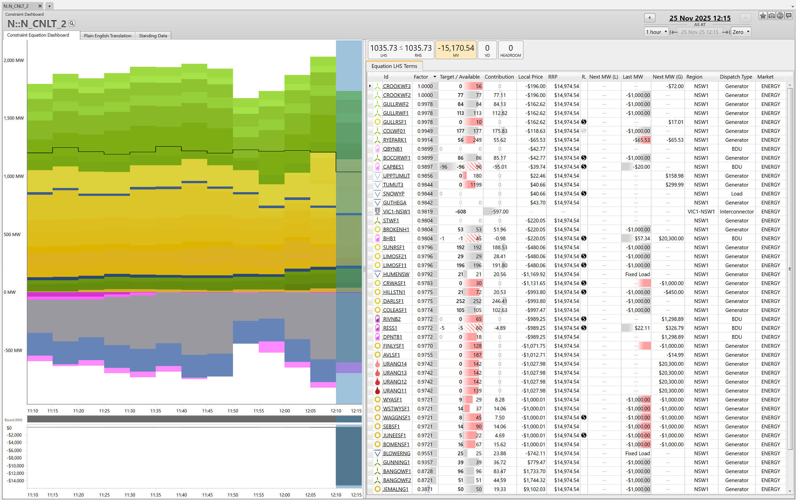
Details of the N::N_CNLT_2 constraint equation during the 12:15 dispatch interval — the interval where the NSW price unexpectedly jumped to $14,974.54/MWh.

Source: ez2view’s Constraint Dashboard. Screenshot taken for the 12:15 dispatch interval.

Looking at the third column from the left in the table in our screenshot above, we can see that many semi-scheduled (i.e. solar and wind) units within the constraint were given very low or even 0 MW targets despite ample availability — indicating that they were being curtailed. As I noted in my article on the day, there were several other constraint equations binding, so some of these units could have been curtailed as a result of those other constraints.

However, curiously we can see that the 100 MW Capital BESS had a target of -96 MW for this interval, meaning that it was instructed to charge/consume at a rate of 96 MW by the end of this interval, at a cost of $14,974.54/MWh.

What happened to the Capital BESS and how did it respond?

If we look at the unit dashboard for the Capital BESS within our ez2view software we can see observe a few details:

• N::N_CNLT_2 was the only constraint equation on whose LHS this unit appeared that actually bound in this dispatch interval.
• The unit’s local price was -$39.74, while the NSW price was $14,974.54.
• We can see that for this dispatch interval, the unit had distributed -48MW of volume in a -$20 price band and -48 MW of volume in a $0 price band. (i.e. both of these bid bands were above the unit’s local price)
• Those volumes had been rebid slightly up from the previous dispatch interval. Effectively, -48 MW of volume was moved from the -$198 price band to $0 price band.

We can therefore gather that the dispatch engine constrained the unit on, as this was the most economic outcome for its solution. In this case, the sudden shift in network flows around NSW meant that additional load from the battery helped relieve the LHS of the N::N_CNLT_2 constraint in order for it to be equal to the equation’s RHS (which had suddenly dropped in this interval, for the theorised reasons we covered above).

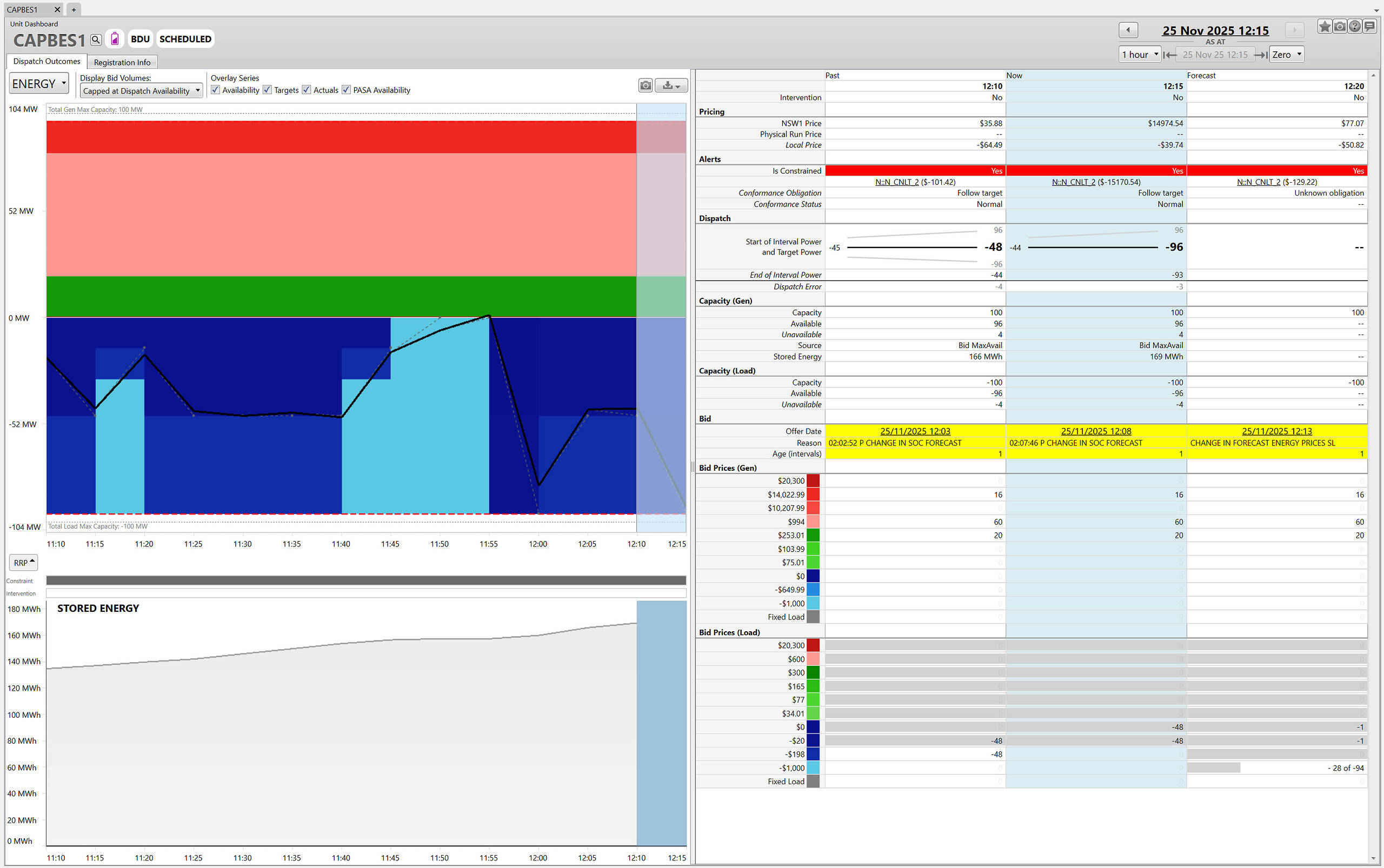
Source: ez2view’s Unit Dashboard. Screenshot taken for the 12:15 dispatch interval.

So what did the battery do next?

In the screenshot below, we see the unit dashboard for Capital BESS in the next interval (the 12:20 dispatch interval). We can see that the battery’s (likely automated) bidder quickly responded by rebidding all of its load volume as unavailable — which resulted in a 0 MW target just as prices jumped to $20,300/MWh, effectively stemming further losses.

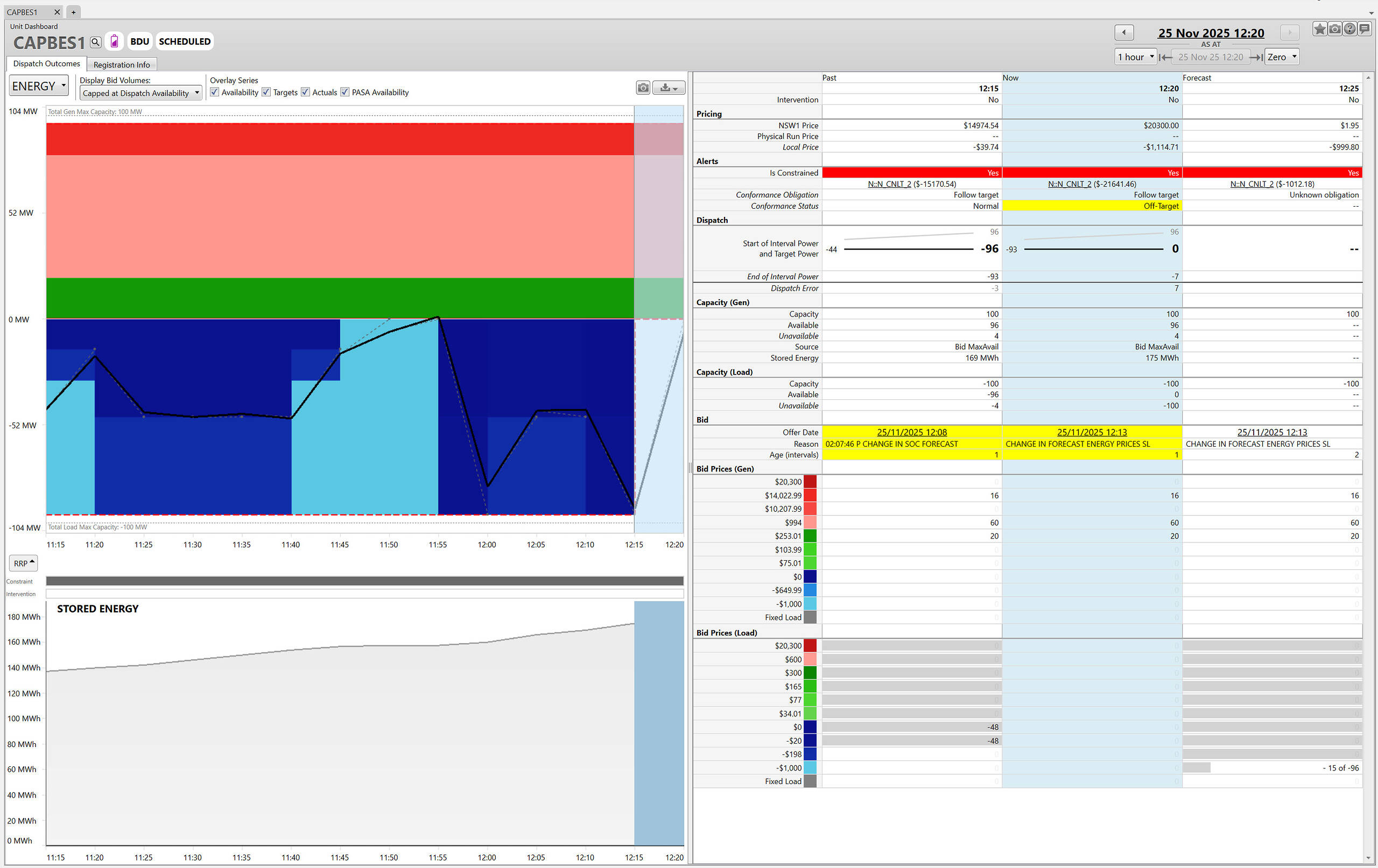
Source: ez2view’s Unit Dashboard. Screenshot taken for the 12:20 dispatch interval.

Hopefully this short case study has helped show that outcomes like this are less a story of a battery “charging at $15,000/MWh!?” and more a glimpse into how the dispatch engine reacts when a sudden, unexpected shift occurs in the grid, and how assets subsequently respond to that reaction.