Spot price arbitrage with battery storage – a review of 2020 performance

As part of the University of Queensland’s energy leadership ambitions, a 1.1 MW / 2.2 MWh Tesla Powerpack battery system was installed constructed at the St Lucia campus in late 2019 – the state’s largest behind-the-meter installation at the time. This coincided with UQ’s move to become the first university in Australia to participate directly in the wholesale electricity spot market as part of the Warwick Solar Farm initiative.

In early 2020, UQ published the Business Case & Q1 2020 Performance Report for the project. This report was well received within the industry, with the document being downloaded over 2,000 times since publication.

Building on this success, a performance review for the full 2020 calendar year has been prepared and can be downloaded here. The following is an extract from the full report, focusing on the battery’s arbitrage function.

As a spot price exposed energy user, one of the core functions of UQ’s battery is to undertake arbitrage – charging to store energy when prices are low and discharging to generate energy when prices are high. UQ’s battery utilises a custom developed control system – the Demand Response Engine (DRE) – to automatically trade in the NEM 24 hours a day, 7 days a week.

 

Financial performance

Net revenue from arbitrage across 2020 totalled just under $45,000. This exceeded business case assumptions by 28% and was primarily a result of realised spreads being higher than forecast. Net revenue by month is shown in Figure 1. Excluding January (which was subject to circumstances driven by natural disasters) this shows an overall trend of increasing arbitrage revenue across the year, with the highest revenue of the year realised in November 2020. On a quarterly basis, Q4 2020 had the highest revenue at $16,500. This is almost double the revenue in each of Q1 2020 and Q2 2020, despite the strong contribution from the month of January.

Figure 2 provides a graphical illustration of cumulative net arbitrage revenue across the year. The line goes up when income is earned from discharging, and down when costs are incurred from charging. Over time, the line would be expected to trend upwards provided the spread in energy price being achieved exceeds the cost associated with roundtrip efficiency losses. Figure 2 shows that while large jumps in net revenue were made on a handful of occasions due to extreme pricing events (such as during January, May, November & December), a slow and steady accumulation of arbitrage revenue from modest spreads throughout the year was equally important in delivering the overall revenue result.

 

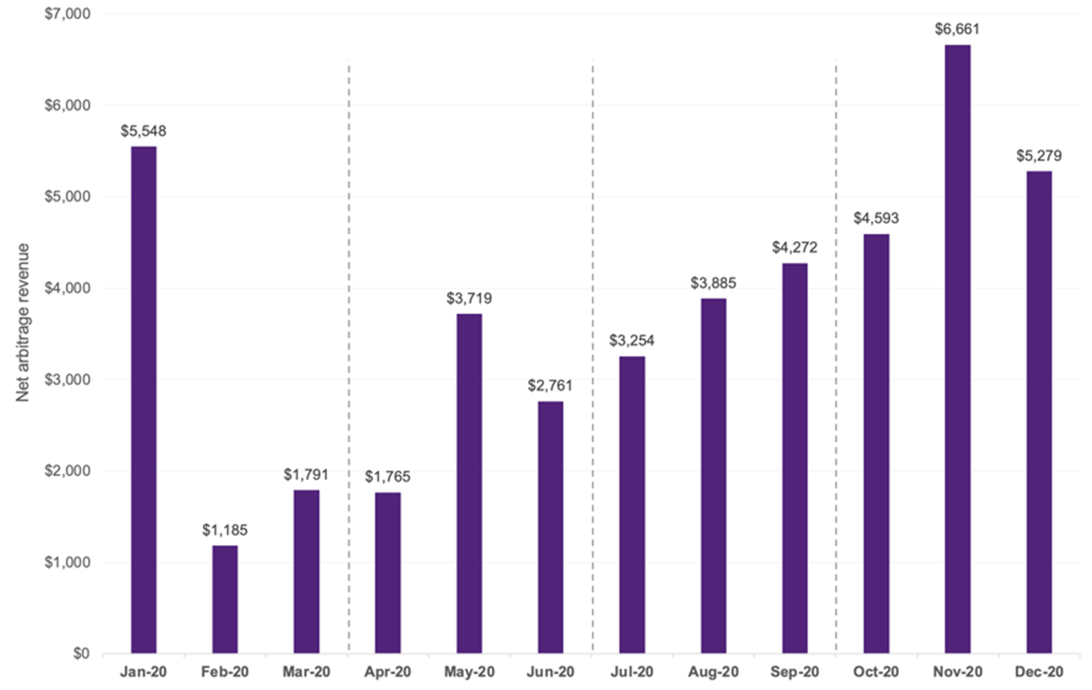Figure 1: Net arbitrage revenue – monthly

 

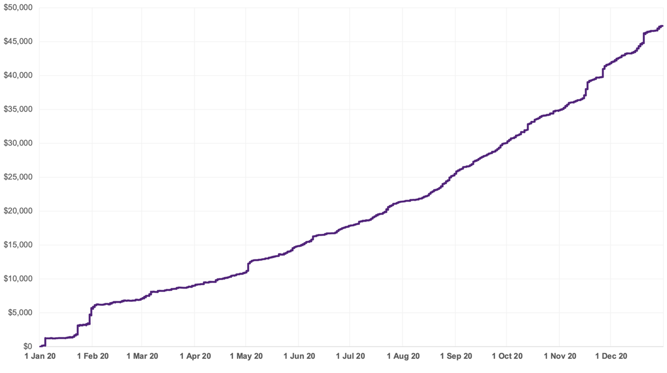Figure 2: Cumulative arbitrage revenue

 

Utilisation analysis

The battery’s utilisation is an important metric for measuring the implementation of the arbitrage service, as well as for ensuring the battery’s operations remain within relevant warranty limits. There are multiple ways that utilisation can be measured, with UQ opting to sum MWh charged plus MWh discharged to create a metric that is measured on an average MWh per day basis. Figure 3 illustrates the daily utilisation factor per month across 2020, with the annual average and warranty limits illustrated. Although warranty limits are based on MWh of discharged energy only, an inferred daily utilisation limit of 4.56 MWh per day can be calculated by adding the equivalent volume of charge energy needed whilst accounting for roundtrip efficiency losses.

As seen in Figure 6, utilisation of the battery steadily increased across the year, with an average utilisation during 2020 of 3.21 MWh per day. This is around 30% below the warranty limit and implies that, on an average basis, UQ’s utilisation of the battery currently has significant headroom to adjust trading strategy. Importantly, even the highest month of utilisation (November) was still almost 8% below the warranty limit (which is assessed on an annual, not monthly basis). The lowest utilisation month (February) had a figure less than half of the warranty limit.

One perspective is that the battery’s ideal utilisation profile would see the daily MWh across the year approach as close to the warranty limit as possible, with the caveat that spreads being achieved must still be sufficient to cover roundtrip efficiency losses, ancillary charges, and any other variable operating costs. Beyond this though, it could be argued that even a net spread of $1/MWh would be preferable to the battery’s capacity being underutilised and zero revenue being realised. This concept is empathised by the previously shown Figure 2 that highlights the important contribution of everyday spreads (versus infrequent price spikes) towards overall arbitrage revenue. Adopting this operational philosophy assumes that the battery owner is happy to accept the forecast degradation curve (guaranteed by warranty), and that sufficient controls could be enacted to ensure that warranty limits are not inadvertently exceeded. This is further complicated by warranty limits being cumulative over the asset life and is an issue that requires a deliberate strategy and continual monitoring. Following the commencement of UQ tracking this metric, the battery’s trading strategy has been gradually adjusted to attempt to increase utilisation, including through a lowering of the minimum spread threshold. This remains an area for future focus and optimisation.

 

Figure 3: Utilisation factor (average daily MWh charged + MWh discharged) – monthly

 

Price analysis

Alongside utilisation, the other key contributor to overall arbitrage revenue is the average spread captured by the battery. The spread is calculated by subtracting the cost of charging from the income earned from discharging. Each of these values are best assessed by converting them to a $/MWh basis.

Figure 4 illustrates the average charge and average discharge price each month across 2020. In total, the average charge price for the year was $16.29/MWh, compared to an average discharge price of $106.63/MWh. This equates to an overall annual spread of $90.34/MWh. Of note, the average charge price during three out of nine months (May, August & September) was negative. This means that the battery was able to take advantage of negative price intervals to such an extent that the overall result for the month was the battery being paid to charge. While not negative, the month of October also saw a very low average charge price ($2.80/MWh). Average discharge prices were highest in January by a large margin as a result of climate and weather driven volatility, however average discharge prices began to climb again during Q4.

 

Figure 4: Average charge and discharge price ($/MWh) – monthly

 

Figure 5 and Figure 6 illustrate a price trend of significant note. Figure 5 shows the average spread achieved by the battery each month compared to the time-weighted Queensland Regional Reference Price (RRP). The RRP is the simple average of the settled price within a region for each trading interval over a period of time and is sometimes also referred to as the ‘flat’ price. This metric has traditionally been one of the most important and widely cited price signals for each region within the NEM. As illustrated in Figure 5, however, a substantial inverse correlation between the battery’s average spread and the QLD RRP can be seen, particularly from Q3 onwards. Figure 6 plots this using the average battery spread as a factor of the QLD RRP. This shows that on average across the year, the battery achieved a spread that was 2.2 times higher than the QLD RRP. In the highest month (September) this factor was just under 3. Most notably, with the exception of January, the highest factors occurred during months where the QLD RRP would be considered ‘low’ by recent comparison. This shows that although average energy prices are now lower than at any point in recent years, there is significant hidden volatility within the headline RRP which is able to be captured by flexible assets such as batteries that can pick out both the highest and lowest priced intervals of each day.

 

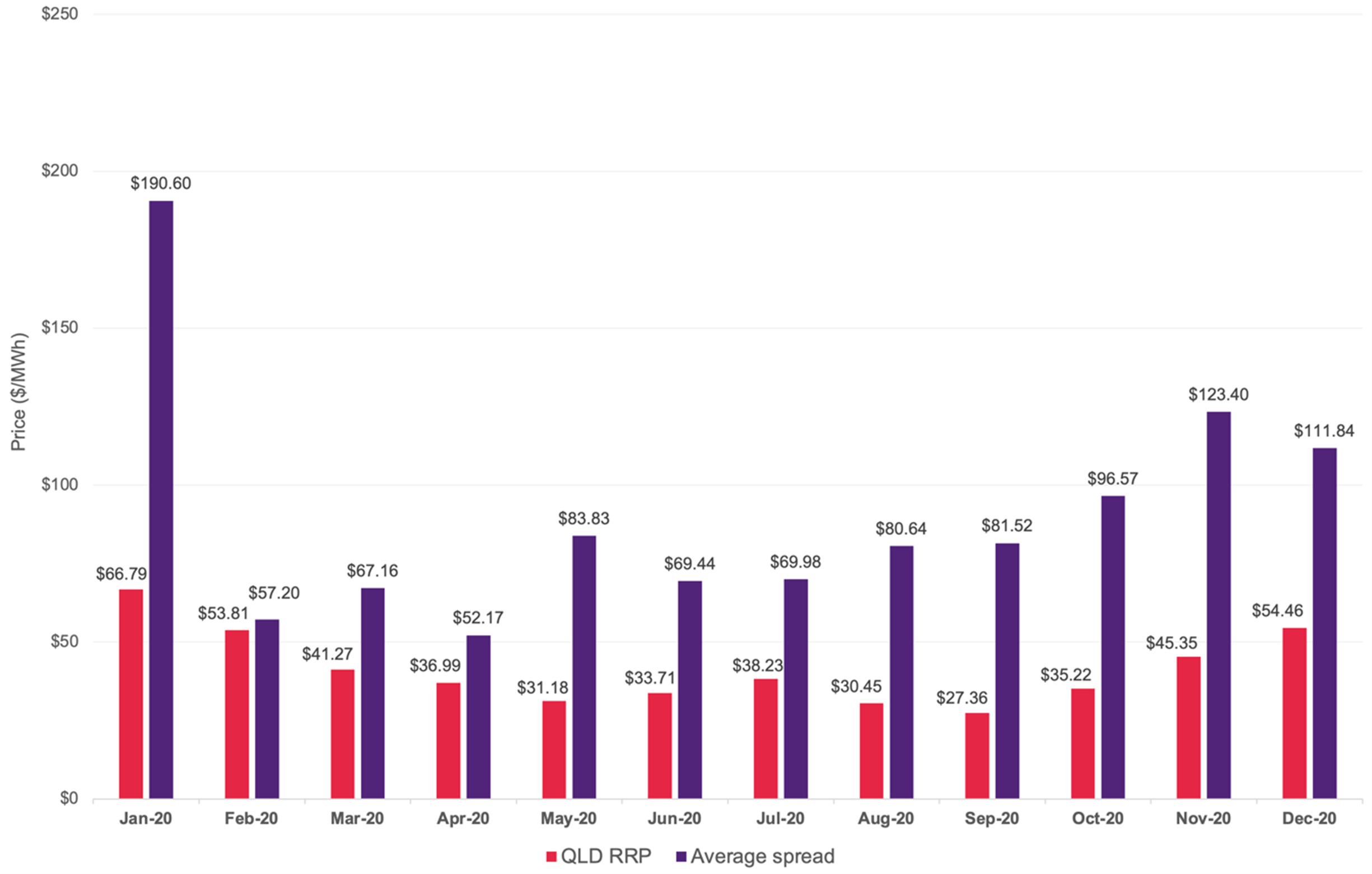Figure 5: QLD RRP vs. average spread – monthly

 

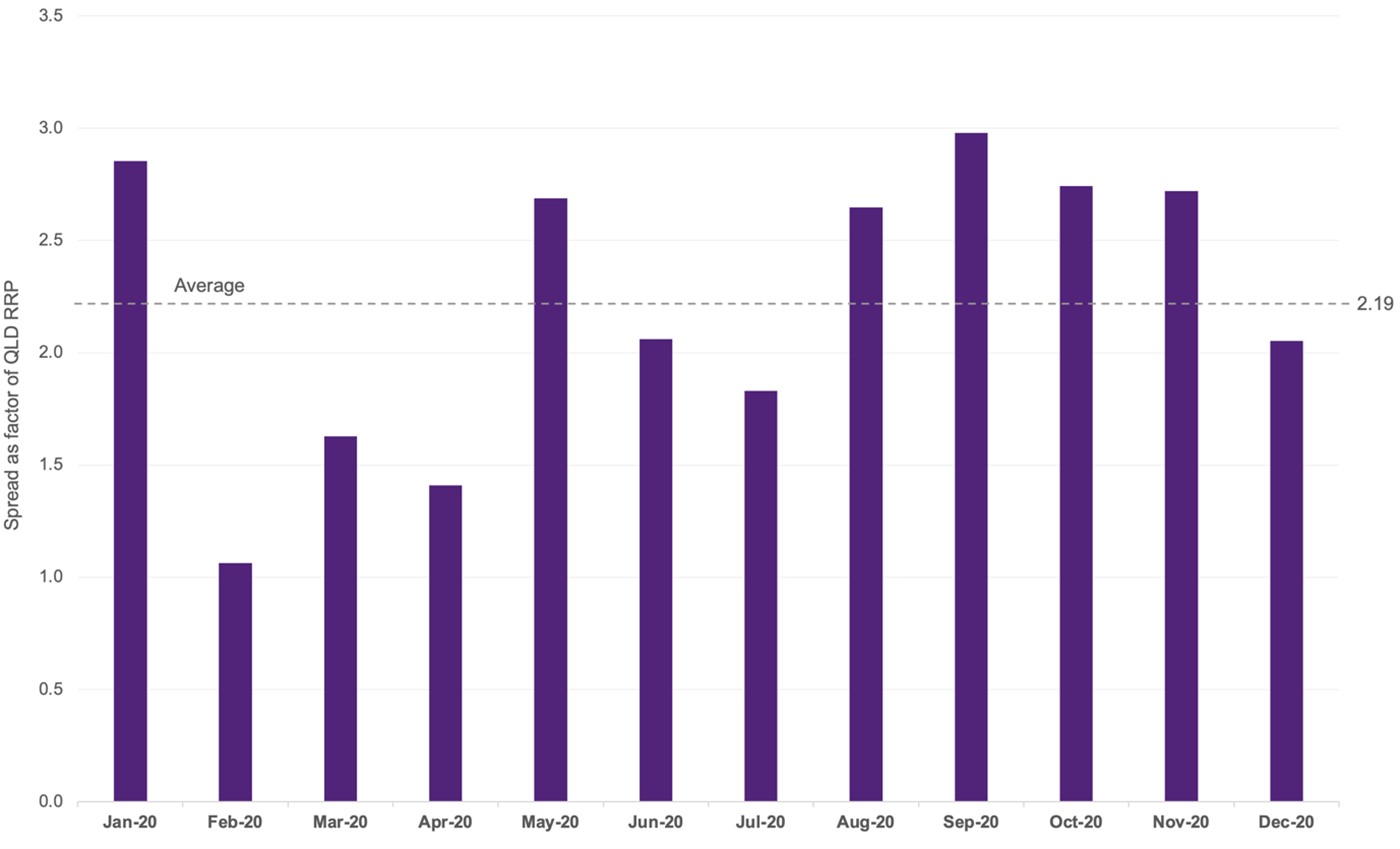Figure 6: Average spread as a factor of QLD RRP – monthly

 

Figure 7 breaks down the portion of income received by the battery each quarter into three price bands – prices higher than $300/MWh, prices between $0/MWh and $300/MWh, and negative priced intervals. This analysis looks only at income received from discharging (or charging if prices were negative) and does not consider the costs of charging. Figure 7 shows a number of interesting trends. Foremost, despite common perceptions about batteries deriving large portions of arbitrage revenue from extremes of pricing (either positive or negative), the majority of income during all quarters came from intervals where prices were within a ‘normal’ range of $0/MWh to $300/MWh. Across the year these intervals contributed 74% of gross income. During Q1, almost 30% of income was derived from prices above $300/MWh, with almost no income from negative prices. During the following quarter, however, this trend was flipped with more than a third of income being derived from negative price intervals. Q3 saw the vast majority of income from the normal price range, whilst >$300/MWh prices returned to being a material contribution to income in Q4. This kind of price band analysis has important ramifications for how battery revenue is forecast, particularly in the context of cap contract valuation, as further discussed in section 5 of the full report. This also highlights the importance of reviewing and updating the control parameters used for arbitrage and other services on at least a quarterly basis.

 

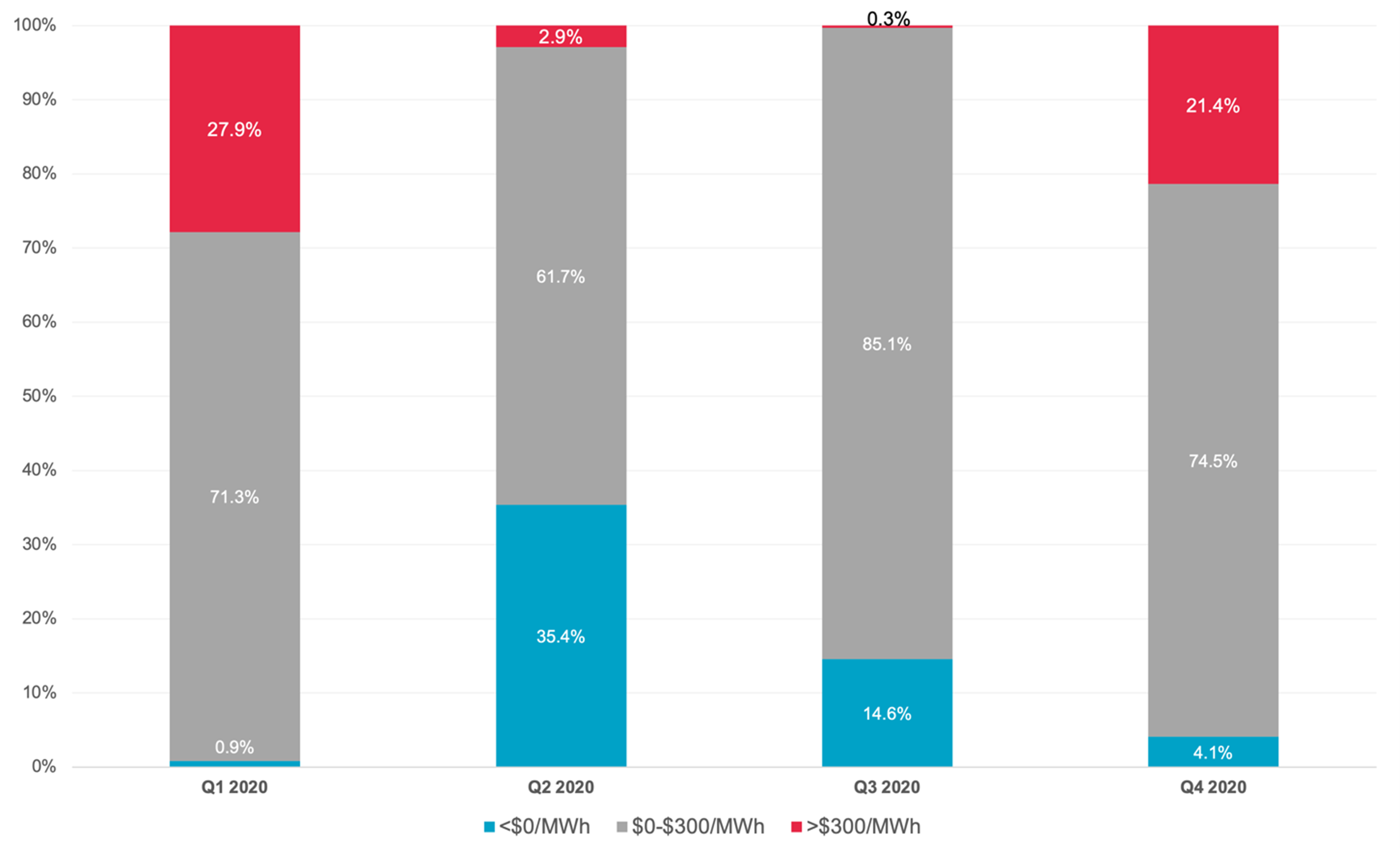Figure 7: Arbitrage gross income by price band – quarterly

 

Perfect forecast vs. actual revenue

Perfect foresight refers to the concept of the maximum possible revenue that could have been earnt by the battery assuming that the control algorithm had complete certainty about spot price outcomes. In reality, arbitrage revenue is partly a function of how well the battery’s control algorithm makes decisions, but more often how accurate the forecasts of pricing being relied upon are. Due to the fact that perfect foresight is never achievable in practice, comparing results from this scenario with actual results is not a fair benchmark. Analysis of the difference between these two values is useful, however, in the context of better understanding how assets like batteries can be modelled. Very little understanding exists in the public domain of the gap between forecast arbitrage revenue based on past or predicted spot pricing and the real-world operational factors that will impact actual results. This ‘discount factor’ between hypothetical maximum income and actual results is a key insight for the prediction of battery project revenue. This analysis can be undertaken in the case of the UQ battery by feeding actual spot price outcomes into the demand response engine algorithm (assuming the same control parameters as existed during 2020) to simulate battery behaviour across the year. This approach has some limitations, such as not being able to account for outages nor discharge during contingency FCAS events, but nonetheless provides a useful reference point regarding the question at hand.

Figure 8 shows the comparison between quarterly arbitrage revenue for the actual versus perfect foresight scenarios. Across the year, the perfect foresight scenario yielded 46.6% more income than what was achieved in reality. Put differently, actual results showed a 31.8% discount compared to perfect foresight. This varied significantly across the year, with perfect foresight showing 80% higher income in Q1, whilst only 25% higher income during Q3. Of note, utilisation of the battery was on average 9.4% higher under the perfect forecast scenario, although this was still well within warranty limits. This suggests that even with perfect foresight, considerable scope exists to tune the battery’s control algorithm to take advantage of smaller but more frequent spreads.

Figure 9 shows the average monthly arbitrage spread achieved in each of the scenarios. Across the year, the perfect foresight scenario achieved an average spread of $116/MWh compared to the actual spread of $90/MWh – a 29% improvement. Significant variation existed between individual months, with the perfect foresight spread in December being 38% higher than actual, while this difference during March was only 12%. The magnitude of spreads between quarters remained consistent in both scenarios however, with Q4 having the highest spreads, whilst Q2 had the lowest. Notably, the perfect foresight scenario achieved a negative average charge price in four out of twelve months compared to three out of twelve months for the actual results, with average charge prices in October tipping into negative in the perfect foresight scenario.

 

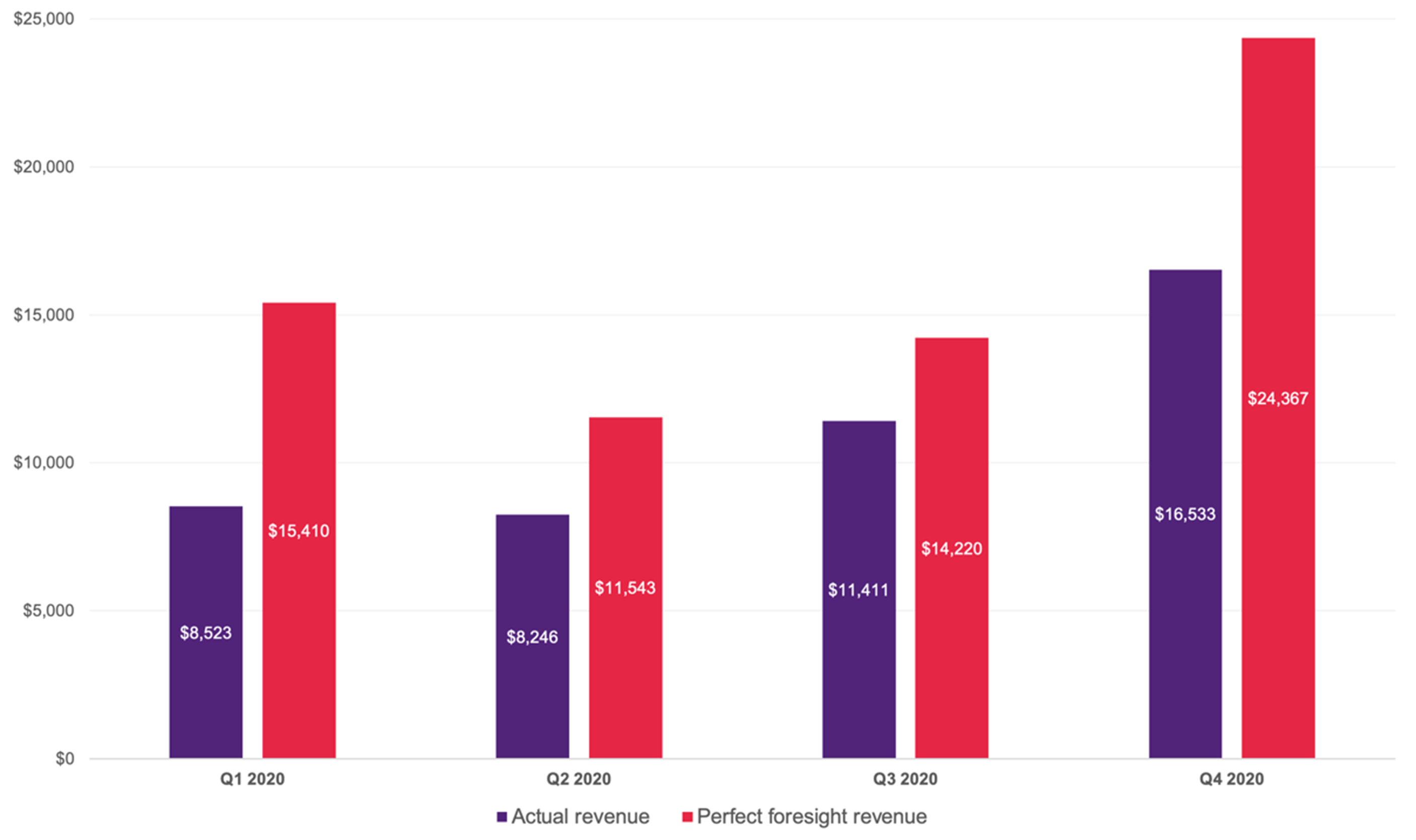Figure 8: Actual vs. perfect foresight arbitrage revenue – quarterly

 

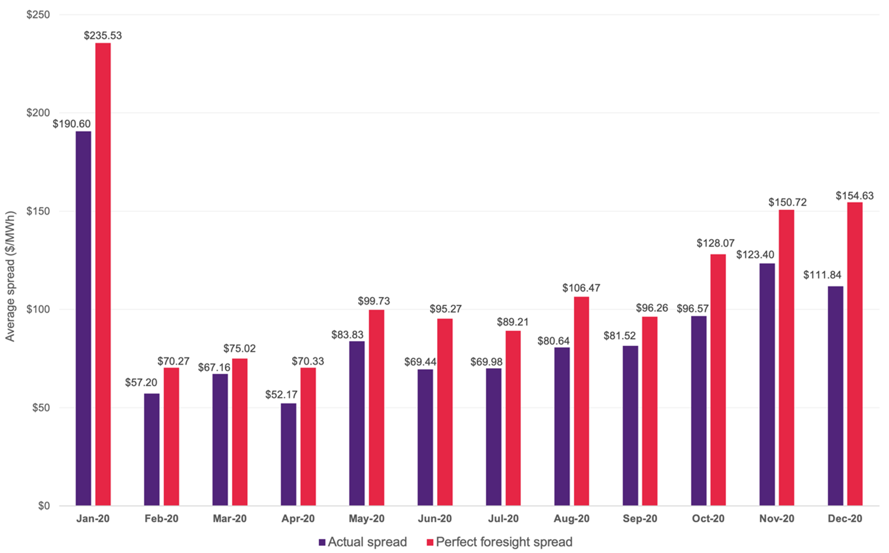Figure 9: Actual vs. perfect foresight average spread ($/MWh) – monthly

 

Ancillary charges

Alongside the direct impact of roundtrip efficiency losses, the other key consideration when assessing arbitrage revenue is the ancillary charges incurred through cycling the battery. These will vary significantly from site to site based on individual network tariffs and market configurations. The following is discussed from UQ’s perspective of operating an asset behind-the-meter at a site with relatively low network charges due to the connection voltage and size of load.

In UQ’s circumstances, ancillary charges derive from the components of the site’s retail electricity bill beyond the simple wholesale cost of the energy used. The ancillary energy charges are levied on a c/kWh basis and include items such as TUOS and DUOS network charges, AEMO market fees, and LGC and STC charges. When charging the battery, UQ incurs additional ancillary energy charges than would otherwise be the case due to the volume of energy measured by the front door meter being increased. When the battery discharges the volume of energy at the front door meter decreases, effectively ‘reimbursing’ UQ for the extra ancillary energy charges that were incurred during charging. These values do not balance out to zero, however, due to the roundtrip efficiency losses of the battery.

Figure 10 provides an illustration of how this works in practice. The first bar shows that when charging, these ancillary charges add up to a gross amount of $27.56/MWh. When UQ discharges this stored energy these same charges are avoided. As the volume of energy discharged is less than the volume charged, only $23.49/MWh of value is returned to UQ. This results in a net ancillary charge of $4.08/MWh. The values presented in Figure 10 are the annual average and are subject to some fluctuation month to month largely due to swings in STC and LGC pricing. These ancillary charges are an unavoidable operating cost of cycling the battery and thus an important input into any calculation of minimum arbitrage spreads required.

 

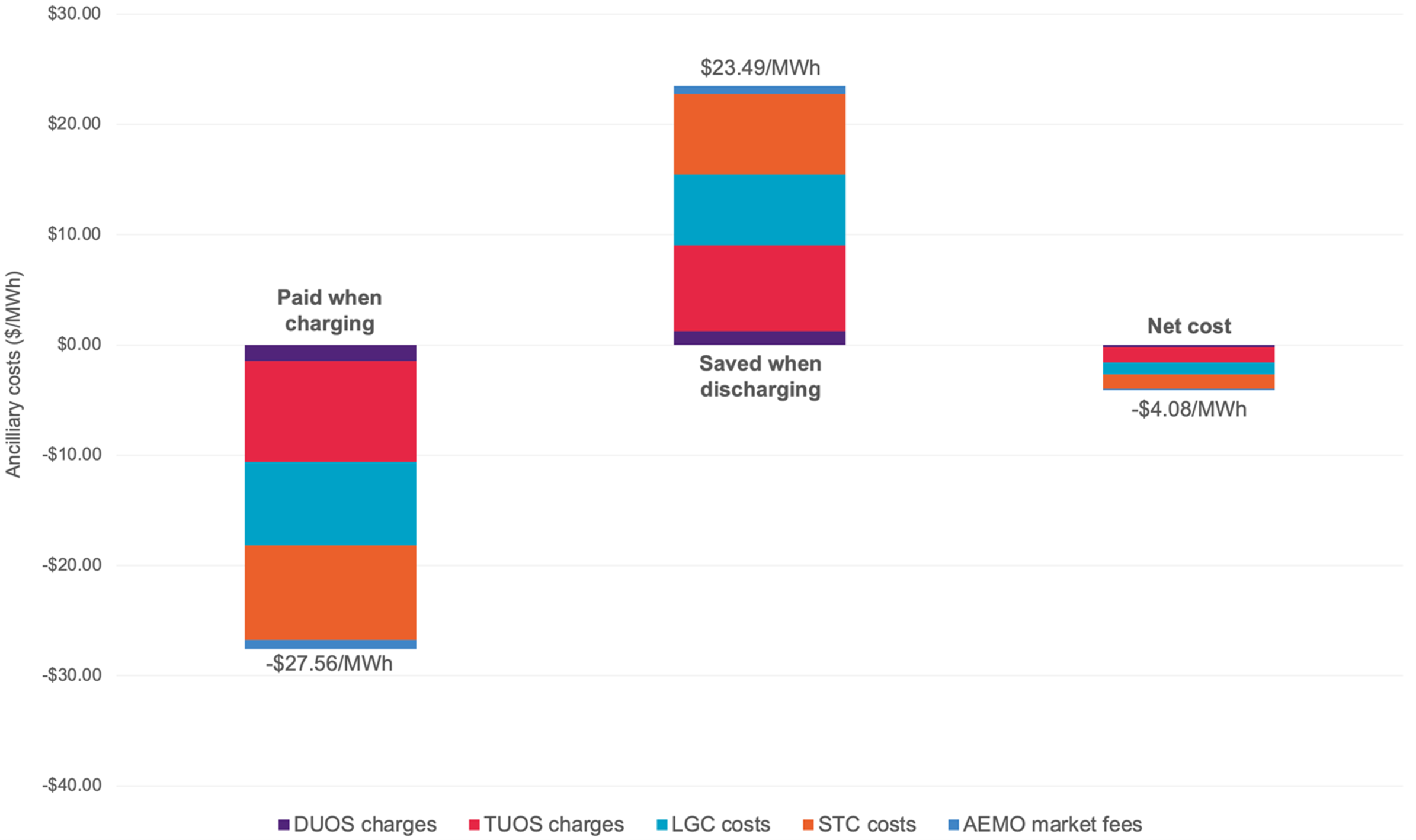Figure 10: Ancillary charges – average $/MWh across year

 

 

Future directions

The arbitrage function is the most well-developed revenue stream for the battery. Notwithstanding this, further opportunities for refinement and improvement exist. As discussed earlier, further work is required to optimise the balance between the minimum spread threshold adopted by the trading algorithm and the desire to maximise utilisation within warranty limits. Considering that on a cumulative basis the battery’s throughput is currently well below warranty limits, this affords a degree of freedom to trial different approaches to this issue. The other primary area of work related to the arbitrage function involves the co-optimisation of this service alongside others, such as FCAS, to ensure the best overall net outcome for the battery during each interval. This is discussed further in section 4 of the full report.

 

————————————–

About our Guest Author